Exponential and Logarithmic Models
We have already explored some basic applications of exponential and logarithmic functions. In this section, we explore some important applications in more depth, including radioactive isotopes and Newton’s Law of Cooling.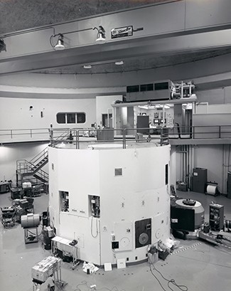 A nuclear research reactor inside the Neely Nuclear Research Center on the Georgia Institute of Technology campus (credit: Georgia Tech Research Institute)
Exponential Growth and Decay
In real-world applications, we need to model the behavior of a function. In mathematical modeling, we choose a familiar general function with properties that suggest that it will model the real-world phenomenon we wish to analyze. In the case of rapid growth, we may choose the exponential growth function:[latex]y={A}_{0}{e}^{kt}[/latex]
where [latex]{A}_{0}[/latex] is equal to the value at time zero, e is Euler’s constant, and k is a positive constant that determines the rate (percentage) of growth. We may use the exponential growth function in applications involving doubling time, the time it takes for a quantity to double. Such phenomena as wildlife populations, financial investments, biological samples, and natural resources may exhibit growth based on a doubling time. In some applications, however, as we will see when we discuss the logistic equation, the logistic model sometimes fits the data better than the exponential model. On the other hand, if a quantity is falling rapidly toward zero, without ever reaching zero, then we should probably choose the exponential decay model. Again, we have the form [latex]y={A}_{0}{e}^{-kt}[/latex] where [latex]{A}_{0}[/latex] is the starting value, and e is Euler’s constant. Now k is a negative constant that determines the rate of decay. We may use the exponential decay model when we are calculating half-life, or the time it takes for a substance to exponentially decay to half of its original quantity. We use half-life in applications involving radioactive isotopes. In our choice of a function to serve as a mathematical model, we often use data points gathered by careful observation and measurement to construct points on a graph and hope we can recognize the shape of the graph. Exponential growth and decay graphs have a distinctive shape, as we can see in the graphs below. It is important to remember that, although parts of each of the two graphs seem to lie on the x-axis, they are really a tiny distance above the x-axis.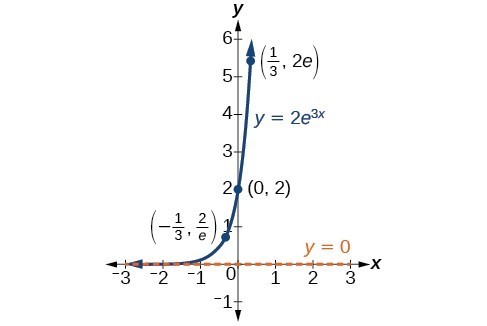 A graph showing exponential growth. The equation is [latex]y=2{e}^{3x}[/latex].
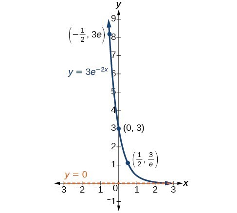 A graph showing exponential decay. The equation is [latex]y=3{e}^{-2x}[/latex].
A General Note: Characteristics of the Exponential Function, [latex]y=A_{0}e^{kt}[/latex]
An exponential function with the form [latex]y={A}_{0}{e}^{kt}[/latex] has the following characteristics:- one-to-one function
- horizontal asymptote: y = 0
- domain: [latex]\left(-\infty , \infty \right)[/latex]
- range: [latex]\left(0,\infty \right)[/latex]
- x intercept: none
- y-intercept: [latex]\left(0,{A}_{0}\right)[/latex]
- increasing if k > 0
- decreasing if k < 0
Try It
The still graphs below include important characteristics of an exponential function that can illustrate whether the function represents growth or decay, and the speed at which the function grows or decays.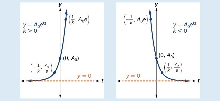 Your task is to add the key features in the still graphs above to the Desmos graph below by using sliders where applicable. The function [latex]f(x) = a\cdot{e}^{kx}[/latex] has been included.
Include the following key features:
Your task is to add the key features in the still graphs above to the Desmos graph below by using sliders where applicable. The function [latex]f(x) = a\cdot{e}^{kx}[/latex] has been included.
Include the following key features:
- The horizontal asymptote
- y-intercept
- The key points labeled in the still graphs above
Example: Graphing Exponential Growth
A population of bacteria doubles every hour. If the culture started with 10 bacteria, graph the population as a function of time.Answer: When an amount grows at a fixed percent per unit time, the growth is exponential. To find [latex]{A}_{0}[/latex] we use the fact that [latex]{A}_{0}[/latex] is the amount at time zero, so [latex]{A}_{0}=10[/latex]. To find k, use the fact that after one hour [latex]\left(t=1\right)[/latex] the population doubles from 10 to 20. The formula is derived as follows
[latex]\begin{array}{l}\text{ }20=10{e}^{k\cdot 1}\hfill & \hfill \\ \text{ }2={e}^{k}\hfill & \text{Divide by 10}\hfill \\ \mathrm{ln}2=k\hfill & \text{Take the natural logarithm}\hfill \end{array}[/latex]
so [latex]k=\mathrm{ln}\left(2\right)[/latex]. Thus the equation we want to graph is [latex]y=10{e}^{\left(\mathrm{ln}2\right)t}=10{\left({e}^{\mathrm{ln}2}\right)}^{t}=10\cdot {2}^{t}[/latex]. The graph is shown below. The graph of [latex]y=10{e}^{\left(\mathrm{ln}2\right)t}[/latex]
 Analysis of the Solution
The population of bacteria after ten hours is 10,240. We could describe this amount is being of the order of magnitude [latex]{10}^{4}[/latex]. The population of bacteria after twenty hours is 10,485,760 which is of the order of magnitude [latex]{10}^{7}[/latex], so we could say that the population has increased by three orders of magnitude in ten hours.Calculating Doubling Time
For growing quantities, we might want to find out how long it takes for a quantity to double. As we mentioned above, the time it takes for a quantity to double is called the doubling time. Given the basic exponential growth equation [latex]A={A}_{0}{e}^{kt}[/latex], doubling time can be found by solving for when the original quantity has doubled, that is, by solving [latex]2{A}_{0}={A}_{0}{e}^{kt}[/latex]. The formula is derived as follows:[latex]\begin{array}{l}2{A}_{0}={A}_{0}{e}^{kt}\hfill & \hfill \\ 2={e}^{kt}\hfill & \text{Divide by }{A}_{0}.\hfill \\ \mathrm{ln}2=kt\hfill & \text{Take the natural logarithm}.\hfill \\ t=\frac{\mathrm{ln}2}{k}\hfill & \text{Divide by the coefficient of }t.\hfill \end{array}[/latex]
Thus the doubling time is[latex]t=\frac{\mathrm{ln}2}{k}[/latex]
Example: Finding a Function That Describes Exponential Growth
According to Moore’s Law, the doubling time for the number of transistors that can be put on a computer chip is approximately two years. Give a function that describes this behavior.Answer: The formula is derived as follows:
[latex]\begin{array}{l}t=\frac{\mathrm{ln}2}{k}\hfill & \text{The doubling time formula}.\hfill \\ 2=\frac{\mathrm{ln}2}{k}\hfill & \text{Use a doubling time of two years}.\hfill \\ k=\frac{\mathrm{ln}2}{2}\hfill & \text{Multiply by }k\text{ and divide by 2}.\hfill \\ A={A}_{0}{e}^{\frac{\mathrm{ln}2}{2}t}\hfill & \text{Substitute }k\text{ into the continuous growth formula}.\hfill \end{array}[/latex]
The function is [latex]A={A}_{0}{e}^{\frac{\mathrm{ln}2}{2}t}[/latex].Try It
Recent data suggests that, as of 2013, the rate of growth predicted by Moore’s Law no longer holds. Growth has slowed to a doubling time of approximately three years. Find the new function that takes that longer doubling time into account.Answer: [latex]f\left(t\right)={A}_{0}{e}^{\frac{\mathrm{ln}2}{3}t}[/latex]
Radiocarbon Dating
The formula for radioactive decay is important in radiocarbon dating, which is used to calculate the approximate date a plant or animal died. Radiocarbon dating was discovered in 1949 by Willard Libby, who won a Nobel Prize for his discovery. It compares the difference between the ratio of two isotopes of carbon in an organic artifact or fossil to the ratio of those two isotopes in the air. It is believed to be accurate to within about 1% error for plants or animals that died within the last 60,000 years. Carbon-14 is a radioactive isotope of carbon that has a half-life of 5,730 years. It occurs in small quantities in the carbon dioxide in the air we breathe. Most of the carbon on Earth is carbon-12, which has an atomic weight of 12 and is not radioactive. Scientists have determined the ratio of carbon-14 to carbon-12 in the air for the last 60,000 years, using tree rings and other organic samples of known dates—although the ratio has changed slightly over the centuries. As long as a plant or animal is alive, the ratio of the two isotopes of carbon in its body is close to the ratio in the atmosphere. When it dies, the carbon-14 in its body decays and is not replaced. By comparing the ratio of carbon-14 to carbon-12 in a decaying sample to the known ratio in the atmosphere, the date the plant or animal died can be approximated. Since the half-life of carbon-14 is 5,730 years, the formula for the amount of carbon-14 remaining after t years is[latex]A\approx {A}_{0}{e}^{\left(\frac{\mathrm{ln}\left(0.5\right)}{5730}\right)t}[/latex]
where- A is the amount of carbon-14 remaining
- [latex]{A}_{0}[/latex] is the amount of carbon-14 when the plant or animal began decaying.
[latex]\begin{array}{l}\text{ }A={A}_{0}{e}^{kt}\hfill & \text{The continuous growth formula}.\hfill \\ \text{ }0.5{A}_{0}={A}_{0}{e}^{k\cdot 5730}\hfill & \text{Substitute the half-life for }t\text{ and }0.5{A}_{0}\text{ for }f\left(t\right).\hfill \\ \text{ }0.5={e}^{5730k}\hfill & \text{Divide by }{A}_{0}.\hfill \\ \mathrm{ln}\left(0.5\right)=5730k\hfill & \text{Take the natural log of both sides}.\hfill \\ \text{ }k=\frac{\mathrm{ln}\left(0.5\right)}{5730}\hfill & \text{Divide by the coefficient of }k.\hfill \\ \text{ }A={A}_{0}{e}^{\left(\frac{\mathrm{ln}\left(0.5\right)}{5730}\right)t}\hfill & \text{Substitute for }r\text{ in the continuous growth formula}.\hfill \end{array}[/latex]
To find the age of an object, we solve this equation for t:[latex]t=\frac{\mathrm{ln}\left(\frac{A}{{A}_{0}}\right)}{-0.000121}[/latex]
Out of necessity, we neglect here the many details that a scientist takes into consideration when doing carbon-14 dating, and we only look at the basic formula. The ratio of carbon-14 to carbon-12 in the atmosphere is approximately 0.0000000001%. Let r be the ratio of carbon-14 to carbon-12 in the organic artifact or fossil to be dated, determined by a method called liquid scintillation. From the equation [latex]A\approx {A}_{0}{e}^{-0.000121t}[/latex] we know the ratio of the percentage of carbon-14 in the object we are dating to the percentage of carbon-14 in the atmosphere is [latex]r=\frac{A}{{A}_{0}}\approx {e}^{-0.000121t}[/latex]. We solve this equation for t, to get[latex]t=\frac{\mathrm{ln}\left(r\right)}{-0.000121}[/latex]
How To: Given the percentage of carbon-14 in an object, determine its age.
- Express the given percentage of carbon-14 as an equivalent decimal, k.
- Substitute for k in the equation [latex]t=\frac{\mathrm{ln}\left(r\right)}{-0.000121}[/latex] and solve for the age, t.
Example: Finding the Age of a Bone
A bone fragment is found that contains 20% of its original carbon-14. To the nearest year, how old is the bone?Answer: We substitute 20% = 0.20 for k in the equation and solve for t:
[latex]\begin{array}{l}t=\frac{\mathrm{ln}\left(r\right)}{-0.000121}\hfill & \text{Use the general form of the equation}.\hfill \\ =\frac{\mathrm{ln}\left(0.20\right)}{-0.000121}\hfill & \text{Substitute for }r.\hfill \\ \approx 13301\hfill & \text{Round to the nearest year}.\hfill \end{array}[/latex]
The bone fragment is about 13,301 years old.Analysis of the Solution
The instruments that measure the percentage of carbon-14 are extremely sensitive and, as we mention above, a scientist will need to do much more work than we did in order to be satisfied. Even so, carbon dating is only accurate to about 1%, so this age should be given as [latex]\text{13,301 years}\pm \text{1% or 13,301 years}\pm \text{133 years}[/latex].Try It
Cesium-137 has a half-life of about 30 years. If we begin with 200 mg of cesium-137, will it take more or less than 230 years until only 1 milligram remains?Answer: less than 230 years, 229.3157 to be exact
[latex]f\left(x\right)=\frac{c}{1+a{e}^{-bx}}[/latex]
The graph below shows how the growth rate changes over time. The graph increases from left to right, but the growth rate only increases until it reaches its point of maximum growth rate, at which point the rate of increase decreases.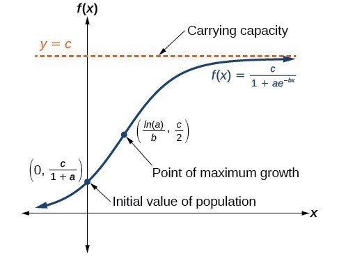
A General Note: Logistic Growth
The logistic growth model is[latex]f\left(x\right)=\frac{c}{1+a{e}^{-bx}}[/latex]
where- [latex]\frac{c}{1+a}[/latex] is the initial value
- c is the carrying capacity, or limiting value
- b is a constant determined by the rate of growth.
Example: Using the Logistic-Growth Model
An influenza epidemic spreads through a population rapidly, at a rate that depends on two factors: The more people who have the flu, the more rapidly it spreads, and also the more uninfected people there are, the more rapidly it spreads. These two factors make the logistic model a good one to study the spread of communicable diseases. And, clearly, there is a maximum value for the number of people infected: the entire population. For example, at time t = 0 there is one person in a community of 1,000 people who has the flu. So, in that community, at most 1,000 people can have the flu. Researchers find that for this particular strain of the flu, the logistic growth constant is b = 0.6030. Estimate the number of people in this community who will have had this flu after ten days. Predict how many people in this community will have had this flu after a long period of time has passed.Answer: We substitute the given data into the logistic growth model
[latex]f\left(x\right)=\frac{c}{1+a{e}^{-bx}}[/latex]
Because at most 1,000 people, the entire population of the community, can get the flu, we know the limiting value is c = 1000. To find a, we use the formula that the number of cases at time t = 0 is [latex]\frac{c}{1+a}=1[/latex], from which it follows that a = 999. This model predicts that, after ten days, the number of people who have had the flu is [latex]f\left(x\right)=\frac{1000}{1+999{e}^{-0.6030x}}\approx 293.8[/latex]. Because the actual number must be a whole number (a person has either had the flu or not) we round to 294. In the long term, the number of people who will contract the flu is the limiting value, c = 1000.Analysis of the Solution
Remember that, because we are dealing with a virus, we cannot predict with certainty the number of people infected. The model only approximates the number of people infected and will not give us exact or actual values. The graph below gives a good picture of how this model fits the data.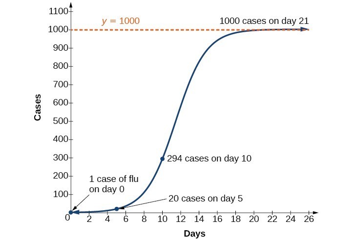 The graph of [latex]f\left(x\right)=\frac{1000}{1+999{e}^{-0.6030x}}[/latex]
Try It
Using the model in the previous example, estimate the number of cases of flu on day 15.Answer: 895 cases on day 15
Choose an Appropriate Model
Now that we have discussed various mathematical models, we need to learn how to choose the appropriate model for the raw data we have. Many factors influence the choice of a mathematical model, among which are experience, scientific laws, and patterns in the data itself. Not all data can be described by elementary functions. Sometimes, a function is chosen that approximates the data over a given interval. For instance, suppose data were gathered on the number of homes bought in the United States from the years 1960 to 2013. After plotting these data in a scatter plot, we notice that the shape of the data from the years 2000 to 2013 follow a logarithmic curve. We could restrict the interval from 2000 to 2010, apply regression analysis using a logarithmic model, and use it to predict the number of home buyers for the year 2015. Three kinds of functions that are often useful in mathematical models are linear functions, exponential functions, and logarithmic functions. If the data lies on a straight line, or seems to lie approximately along a straight line, a linear model may be best. If the data is non-linear, we often consider an exponential or logarithmic model, though other models, such as quadratic models, may also be considered. In choosing between an exponential model and a logarithmic model, we look at the way the data curves. This is called the concavity. If we draw a line between two data points, and all (or most) of the data between those two points lies above that line, we say the curve is concave down. We can think of it as a bowl that bends downward and therefore cannot hold water. If all (or most) of the data between those two points lies below the line, we say the curve is concave up. In this case, we can think of a bowl that bends upward and can therefore hold water. An exponential curve, whether rising or falling, whether representing growth or decay, is always concave up away from its horizontal asymptote. A logarithmic curve is always concave away from its vertical asymptote. In the case of positive data, which is the most common case, an exponential curve is always concave up, and a logarithmic curve always concave down. A logistic curve changes concavity. It starts out concave up and then changes to concave down beyond a certain point, called a point of inflection. After using the graph to help us choose a type of function to use as a model, we substitute points, and solve to find the parameters. We reduce round-off error by choosing points as far apart as possible.Example: Choosing a Mathematical Model
Does a linear, exponential, logarithmic, or logistic model best fit the values listed below? Find the model, and use a graph to check your choice.| x | 1 | 2 | 3 | 4 | 5 | 6 | 7 | 8 | 9 |
| y | 0 | 1.386 | 2.197 | 2.773 | 3.219 | 3.584 | 3.892 | 4.159 | 4.394 |
Answer:
First, plot the data on a graph as in the graph below. For the purpose of graphing, round the data to two significant digits.
 Clearly, the points do not lie on a straight line, so we reject a linear model. If we draw a line between any two of the points, most or all of the points between those two points lie above the line, so the graph is concave down, suggesting a logarithmic model. We can try [latex]y=a\mathrm{ln}\left(bx\right)[/latex]. Plugging in the first point, [latex]\left(\text{1,0}\right)[/latex], gives [latex]0=a\mathrm{ln}b[/latex]. We reject the case that a = 0 (if it were, all outputs would be 0), so we know
[latex]\mathrm{ln}\left(b\right)=0[/latex]. Thus b = 1 and [latex]y=a\mathrm{ln}\left(\text{x}\right)[/latex]. Next we can use the point [latex]\left(\text{9,4}\text{.394}\right)[/latex] to solve for a: [latex]\begin{array}{l}y=a\mathrm{ln}\left(x\right)\hfill \\ 4.394=a\mathrm{ln}\left(9\right)\hfill \\ a=\frac{4.394}{\mathrm{ln}\left(9\right)}\hfill \end{array}[/latex]
Because [latex]a=\frac{4.394}{\mathrm{ln}\left(9\right)}\approx 2[/latex], an appropriate model for the data is [latex]y=2\mathrm{ln}\left(x\right)[/latex]. To check the accuracy of the model, we graph the function together with the given points. The graph of [latex]y=2\mathrm{ln}x[/latex].
 The graph of [latex]y=\mathrm{ln}\left({x}^{2}\right)[/latex]
Try It
Does a linear, exponential, or logarithmic model best fit the data in the table below? Find the model.| x | 1 | 2 | 3 | 4 | 5 | 6 | 7 | 8 | 9 |
| y | 3.297 | 5.437 | 8.963 | 14.778 | 24.365 | 40.172 | 66.231 | 109.196 | 180.034 |
Answer: Exponential. [latex]y=2{e}^{0.5x}[/latex].
Expressing an Exponential Model in Base e
While powers and logarithms of any base can be used in modeling, the two most common bases are [latex]10[/latex] and [latex]e[/latex]. In science and mathematics, the base e is often preferred. We can use laws of exponents and laws of logarithms to change any base to base e.How To: Given a model with the form [latex]y=a{b}^{x}[/latex], change it to the form [latex]y={A}_{0}{e}^{kx}[/latex].
- Rewrite [latex]y=a{b}^{x}[/latex] as [latex]y=a{e}^{\mathrm{ln}\left({b}^{x}\right)}[/latex].
- Use the power rule of logarithms to rewrite y as [latex]y=a{e}^{x\mathrm{ln}\left(b\right)}=a{e}^{\mathrm{ln}\left(b\right)x}[/latex].
- Note that [latex]a={A}_{0}[/latex] and [latex]k=\mathrm{ln}\left(b\right)[/latex] in the equation [latex]y={A}_{0}{e}^{kx}[/latex].
Example: Changing to base e
Change the function [latex]y=2.5{\left(3.1\right)}^{x}[/latex] so that this same function is written in the form [latex]y={A}_{0}{e}^{kx}[/latex].Answer: The formula is derived as follows
[latex]\begin{array}{l}y=2.5{\left(3.1\right)}^{x}\hfill & \hfill \\ =2.5{e}^{\mathrm{ln}\left({3.1}^{x}\right)}\hfill & \text{Insert exponential and its inverse}\text{.}\hfill \\ =2.5{e}^{x\mathrm{ln}3.1}\hfill & \text{Laws of logs}\text{.}\hfill \\ =2.5{e}^{\left(\mathrm{ln}3.1\right)}{}^{x}\hfill & \text{Commutative law of multiplication}\hfill \end{array}[/latex]
Try It
Change the function [latex]y=3{\left(0.5\right)}^{x}[/latex] to one having e as the base.Answer: [latex]y=3{e}^{\left(\mathrm{ln}0.5\right)x}[/latex]
Exponential Regression
As we’ve learned, there are a multitude of situations that can be modeled by exponential functions, such as investment growth, radioactive decay, atmospheric pressure changes, and temperatures of a cooling object. What do these phenomena have in common? For one thing, all the models either increase or decrease as time moves forward. But that’s not the whole story. It’s the way data increase or decrease that helps us determine whether it is best modeled by an exponential equation. Knowing the behavior of exponential functions in general allows us to recognize when to use exponential regression, so let’s review exponential growth and decay. Recall that exponential functions have the form [latex]y=a{b}^{x}[/latex] or [latex]y={A}_{0}{e}^{kx}[/latex]. When performing regression analysis, we use the form most commonly used on graphing utilities, [latex]y=a{b}^{x}[/latex]. Take a moment to reflect on the characteristics we’ve already learned about the exponential function [latex]y=a{b}^{x}[/latex] (assume a > 0):- b must be greater than zero and not equal to one.
- The initial value of the model is y = a.
- If b > 1, the function models exponential growth. As x increases, the outputs of the model increase slowly at first, but then increase more and more rapidly, without bound.
- If 0 < b < 1, the function models exponential decay. As x increases, the outputs for the model decrease rapidly at first and then level off to become asymptotic to the x-axis. In other words, the outputs never become equal to or less than zero.
A General Note: Exponential Regression
Exponential regression is used to model situations in which growth begins slowly and then accelerates rapidly without bound, or where decay begins rapidly and then slows down to get closer and closer to zero. We use the command "ExpReg" on a graphing utility to fit an exponential function to a set of data points. This returns an equation of the form, [latex]y=a{b}^{x}[/latex] Note that:- b must be non-negative.
- when b > 1, we have an exponential growth model.
- when 0 < b < 1, we have an exponential decay model.
How To: Given a set of data, perform exponential regression using a graphing utility.
- Use the STAT then EDIT menu to enter given data.
- Clear any existing data from the lists.
- List the input values in the L1 column.
- List the output values in the L2 column.
- Graph and observe a scatter plot of the data using the STATPLOT feature.
- Use ZOOM [9] to adjust axes to fit the data.
- Verify the data follow an exponential pattern.
- Find the equation that models the data.
- Select "ExpReg" from the STAT then CALC menu.
- Use the values returned for a and b to record the model, [latex]y=a{b}^{x}[/latex].
- Graph the model in the same window as the scatterplot to verify it is a good fit for the data.
Example: Using Exponential Regression to Fit a Model to Data
In 2007, a university study was published investigating the crash risk of alcohol impaired driving. Data from 2,871 crashes were used to measure the association of a person’s blood alcohol level (BAC) with the risk of being in an accident. The table below shows results from the study.[footnote]Source: Indiana University Center for Studies of Law in Action, 2007[/footnote] The relative risk is a measure of how many times more likely a person is to crash. So, for example, a person with a BAC of 0.09 is 3.54 times as likely to crash as a person who has not been drinking alcohol.| BAC | 0 | 0.01 | 0.03 | 0.05 | 0.07 | 0.09 |
| Relative Risk of Crashing | 1 | 1.03 | 1.06 | 1.38 | 2.09 | 3.54 |
| BAC | 0.11 | 0.13 | 0.15 | 0.17 | 0.19 | 0.21 |
| Relative Risk of Crashing | 6.41 | 12.6 | 22.1 | 39.05 | 65.32 | 99.78 |
- Let x represent the BAC level, and let y represent the corresponding relative risk. Use exponential regression to fit a model to these data.
- After 6 drinks, a person weighing 160 pounds will have a BAC of about 0.16. How many times more likely is a person with this weight to crash if they drive after having a 6-pack of beer? Round to the nearest hundredth.
Answer:
- Using the STAT then EDIT menu on a graphing utility, list the BAC values in L1 and the relative risk values in L2. Then use the STATPLOT feature to verify that the scatterplot follows the exponential pattern:
 Use the "ExpReg" command from the STAT then CALC menu to obtain the exponential model,
[latex]y=0.58304829{\left(2.20720213\text{E}10\right)}^{x}[/latex]
Converting from scientific notation, we have:[latex]y=0.58304829{\left(\text{22,072,021,300}\right)}^{x}[/latex]
Notice that [latex]{r}^{2}\approx 0.97[/latex] which indicates the model is a good fit to the data. To see this, graph the model in the same window as the scatterplot to verify it is a good fit:
- Use the model to estimate the risk associated with a BAC of 0.16. Substitute 0.16 for x in the model and solve for y.
[latex]\begin{array}{l}y\hfill & =0.58304829{\left(\text{22,072,021,300}\right)}^{x}\hfill & \text{Use the regression model found in part (a)}\text{.}\hfill \\ \hfill & =0.58304829{\left(\text{22,072,021,300}\right)}^{0.16}\hfill & \text{Substitute 0}\text{.16 for }x\text{.}\hfill \\ \hfill & \approx \text{26}\text{.35}\hfill & \text{Round to the nearest hundredth}\text{.}\hfill \end{array}[/latex]
If a 160-pound person drives after having 6 drinks, he or she is about 26.35 times more likely to crash than if driving while sober.
Try It
The table below shows a recent graduate’s credit card balance each month after graduation.| Month | 1 | 2 | 3 | 4 | 5 | 6 | 7 | 8 |
| Debt ($) | 620.00 | 761.88 | 899.80 | 1039.93 | 1270.63 | 1589.04 | 1851.31 | 2154.92 |
- Use exponential regression to fit a model to these data.
- If spending continues at this rate, what will the graduate’s credit card debt be one year after graduating?
Answer:
- The exponential regression model that fits these data is [latex]y=522.88585984{\left(1.19645256\right)}^{x}[/latex].
- If spending continues at this rate, the graduate’s credit card debt will be $4,499.38 after one year.
Q & A
Is it reasonable to assume that an exponential regression model will represent a situation indefinitely?
No. Remember that models are formed by real-world data gathered for regression. It is usually reasonable to make estimates within the interval of original observation (interpolation). However, when a model is used to make predictions, it is important to use reasoning skills to determine whether the model makes sense for inputs far beyond the original observation interval (extrapolation).Key Equations
| Half-life formula | If [latex]\text{ }A={A}_{0}{e}^{kt}[/latex], k < 0, the half-life is [latex]t=-\frac{\mathrm{ln}\left(2\right)}{k}[/latex]. |
| Carbon-14 dating | [latex]t=\frac{\mathrm{ln}\left(\frac{A}{{A}_{0}}\right)}{-0.000121}[/latex].[latex]{A}_{0}[/latex] A is the amount of carbon-14 when the plant or animal died t is the amount of carbon-14 remaining today is the age of the fossil in years |
| Doubling time formula | If [latex]A={A}_{0}{e}^{kt}[/latex], k > 0, the doubling time is [latex]t=\frac{\mathrm{ln}2}{k}[/latex] |
| Newton’s Law of Cooling | [latex]T\left(t\right)=A{e}^{kt}+{T}_{s}[/latex], where [latex]{T}_{s}[/latex] is the ambient temperature, [latex]A=T\left(0\right)-{T}_{s}[/latex], and k is the continuous rate of cooling. |
Key Concepts
- The basic exponential function is [latex]f\left(x\right)=a{b}^{x}[/latex]. If b > 1, we have exponential growth; if 0 < b < 1, we have exponential decay.
- We can also write this formula in terms of continuous growth as [latex]A={A}_{0}{e}^{kx}[/latex], where [latex]{A}_{0}[/latex] is the starting value. If [latex]{A}_{0}[/latex] is positive, then we have exponential growth when k > 0 and exponential decay when k < 0.
- In general, we solve problems involving exponential growth or decay in two steps. First, we set up a model and use the model to find the parameters. Then we use the formula with these parameters to predict growth and decay.
- We can find the age, t, of an organic artifact by measuring the amount, k, of carbon-14 remaining in the artifact and using the formula [latex]t=\frac{\mathrm{ln}\left(k\right)}{-0.000121}[/latex] to solve for t.
- Given a substance’s doubling time or half-time, we can find a function that represents its exponential growth or decay.
- We can use Newton’s Law of Cooling to find how long it will take for a cooling object to reach a desired temperature, or to find what temperature an object will be after a given time.
- We can use logistic growth functions to model real-world situations where the rate of growth changes over time, such as population growth, spread of disease, and spread of rumors.
- We can use real-world data gathered over time to observe trends. Knowledge of linear, exponential, logarithmic, and logistic graphs help us to develop models that best fit our data.
- Any exponential function with the form [latex]y=a{b}^{x}[/latex] can be rewritten as an equivalent exponential function with the form [latex]y={A}_{0}{e}^{kx}[/latex] where [latex]k=\mathrm{ln}b[/latex].
- Exponential regression is used to model situations where growth begins slowly and then accelerates rapidly without bound, or where decay begins rapidly and then slows down to get closer and closer to zero.
Glossary
carrying capacity in a logistic model, the limiting value of the output doubling time the time it takes for a quantity to double half-life the length of time it takes for a substance to exponentially decay to half of its original quantity logistic growth model a function of the form [latex]f\left(x\right)=\frac{c}{1+a{e}^{-bx}}[/latex] where [latex]\frac{c}{1+a}[/latex] is the initial value, c is the carrying capacity, or limiting value, and b is a constant determined by the rate of growth Newton’s Law of Cooling the scientific formula for temperature as a function of time as an object’s temperature is equalized with the ambient temperature order of magnitude the power of ten, when a number is expressed in scientific notation, with one non-zero digit to the left of the decimalLicenses & Attributions
CC licensed content, Original
- Revision and Adaptation. Provided by: Lumen Learning License: CC BY: Attribution.
- Exponential Growth and Decay Interactive. Authored by: Lumen Learning. Located at: https://www.desmos.com/calculator/4zae7vnjfr. License: Public Domain: No Known Copyright.
CC licensed content, Shared previously
- Precalculus. Provided by: OpenStax Authored by: Jay Abramson, et al.. Located at: https://openstax.org/books/precalculus/pages/1-introduction-to-functions. License: CC BY: Attribution. License terms: Download For Free at : http://cnx.org/contents/[email protected]..
- College Algebra. Provided by: OpenStax Authored by: Abramson, Jay et al.. License: CC BY: Attribution. License terms: Download for free at http://cnx.org/contents/[email protected].
- Question ID 29686. Authored by: McClure, Caren. License: CC BY: Attribution. License terms: IMathAS Community License CC-BY + GPL.
- Question ID 100026. Authored by: Rieman, Rick. License: CC BY: Attribution. License terms: IMathAS Community License CC-BY + GPL.
- Question ID 5801. Authored by: David Lippman. License: CC BY: Attribution. License terms: IMathAS Community License CC-BY + GPL.
