Substitution with Definite Integrals
Learning Objectives
- Use substitution to evaluate definite integrals.
Substitution for Definite Integrals
Substitution can be used with definite integrals, too. However, using substitution to evaluate a definite integral requires a change to the limits of integration. If we change variables in the integrand, the limits of integration change as well.
Substitution with Definite Integrals
Let [latex]u=g(x)[/latex] and let [latex]{g}^{\text{′}}[/latex] be continuous over an interval [latex]\left[a,b\right],[/latex] and let [latex]f[/latex] be continuous over the range of [latex]u=g(x).[/latex] Then,
Although we will not formally prove this theorem, we justify it with some calculations here. From the substitution rule for indefinite integrals, if [latex]F(x)[/latex] is an antiderivative of [latex]f(x),[/latex] we have
Then
and we have the desired result.
Using Substitution to Evaluate a Definite Integral
Use substitution to evaluate [latex]{\int }_{0}^{1}{x}^{2}{(1+2{x}^{3})}^{5}dx.[/latex]
Answer:
Let [latex]u=1+2{x}^{3},[/latex] so [latex]du=6{x}^{2}dx.[/latex] Since the original function includes one factor of [latex]x[/latex]2 and [latex]du=6{x}^{2}dx,[/latex] multiply both sides of the du equation by [latex]1\text{/}6.[/latex] Then,
To adjust the limits of integration, note that when [latex]x=0,u=1+2(0)=1,[/latex] and when [latex]x=1,u=1+2(1)=3.[/latex] Then
Evaluating this expression, we get
Use substitution to evaluate the definite integral [latex]{\int }_{-1}^{0}y{(2{y}^{2}-3)}^{5}dy.[/latex]
Answer:
[latex]\frac{91}{3}[/latex]
Using Substitution with an Exponential Function
Use substitution to evaluate [latex]{\int }_{0}^{1}x{e}^{4{x}^{2}+3}dx.[/latex]
Answer:
Let [latex]u=4{x}^{3}+3.[/latex] Then, [latex]du=8xdx.[/latex] To adjust the limits of integration, we note that when [latex]x=0,u=3,[/latex] and when [latex]x=1,u=7.[/latex] So our substitution gives
Use substitution to evaluate [latex]{\int }_{0}^{1}{x}^{2} \cos (\frac{\pi }{2}{x}^{3})dx.[/latex]
Answer:
[latex]\frac{2}{3\pi }\approx 0.2122[/latex]
Substitution may be only one of the techniques needed to evaluate a definite integral. All of the properties and rules of integration apply independently, and trigonometric functions may need to be rewritten using a trigonometric identity before we can apply substitution. Also, we have the option of replacing the original expression for [latex]u[/latex] after we find the antiderivative, which means that we do not have to change the limits of integration. These two approaches are shown in (Figure).
Using Substitution to Evaluate a Trigonometric Integral
Use substitution to evaluate [latex]{\int }_{0}^{\pi \text{/}2}{ \cos }^{2}\theta d\theta .[/latex]
Answer:
Let us first use a trigonometric identity to rewrite the integral. The trig identity [latex]{ \cos }^{2}\theta =\frac{1+ \cos 2\theta }{2}[/latex] allows us to rewrite the integral as
Then,
We can evaluate the first integral as it is, but we need to make a substitution to evaluate the second integral. Let [latex]u=2\theta .[/latex] Then, [latex]du=2d\theta ,[/latex] or [latex]\frac{1}{2}du=d\theta .[/latex] Also, when [latex]\theta =0,u=0,[/latex] and when [latex]\theta =\pi \text{/}2,u=\pi .[/latex] Expressing the second integral in terms of [latex]u[/latex], we have
Evaluating a Definite Integral Involving an Exponential Function
Evaluate the definite integral [latex]{\int }_{1}^{2}{e}^{1-x}dx.[/latex]
Answer:
Again, substitution is the method to use. Let [latex]u=1-x,[/latex] so [latex]du=-1dx[/latex] or [latex]\text{−}du=dx.[/latex] Then [latex]\int {e}^{1-x}dx=\text{−}\int {e}^{u}du.[/latex] Next, change the limits of integration. Using the equation [latex]u=1-x,[/latex] we have
The integral then becomes
See (Figure).
![A graph of the function f(x) = e^(1-x) over [0, 3]. It crosses the y axis at (0, e) as a decreasing concave up curve and symptotically approaches 0 as x goes to infinity.](https://s3-us-west-2.amazonaws.com/courses-images/wp-content/uploads/sites/2332/2018/01/11204254/CNX_Calc_Figure_05_06_002.jpg) Figure 2. The indicated area can be calculated by evaluating a definite integral using substitution.
Figure 2. The indicated area can be calculated by evaluating a definite integral using substitution.Evaluate [latex]{\int }_{0}^{2}{e}^{2x}dx.[/latex]
Answer:
[latex]\frac{1}{2}{\int }_{0}^{4}{e}^{u}du=\frac{1}{2}({e}^{4}-1)[/latex]
Evaluating a Definite Integral Using Substitution
Evaluate the definite integral using substitution: [latex]{\int }_{1}^{2}\frac{{e}^{1\text{/}x}}{{x}^{2}}dx.[/latex]
Answer:
This problem requires some rewriting to simplify applying the properties. First, rewrite the exponent on [latex]e[/latex] as a power of [latex]x[/latex], then bring the [latex]x[/latex]2 in the denominator up to the numerator using a negative exponent. We have
Let [latex]u={x}^{-1},[/latex] the exponent on [latex]e[/latex]. Then
Bringing the negative sign outside the integral sign, the problem now reads
Next, change the limits of integration:
Evaluate the definite integral using substitution: [latex]{\int }_{1}^{2}\frac{1}{{x}^{3}}{e}^{4{x}^{-2}}dx.[/latex]
Answer:
[latex]{\int }_{1}^{2}\frac{1}{{x}^{3}}{e}^{4{x}^{-2}}dx=\frac{1}{8}\left[{e}^{4}-e\right][/latex]
Hint
Let [latex]u=4{x}^{-2}.[/latex]
(Figure) is a definite integral of a trigonometric function. With trigonometric functions, we often have to apply a trigonometric property or an identity before we can move forward. Finding the right form of the integrand is usually the key to a smooth integration.
Evaluating a Definite Integral
Find the definite integral of [latex]{\int }_{0}^{\pi \text{/}2}\frac{ \sin x}{1+ \cos x}dx.[/latex]
Answer:
We need substitution to evaluate this problem. Let [latex]u=1+ \cos x,,[/latex] so [latex]du=\text{−} \sin xdx.[/latex] Rewrite the integral in terms of [latex]u[/latex], changing the limits of integration as well. Thus,
Then
Evaluating a Definite Integral Using Inverse Trigonometric Functions
Evaluate the definite integral [latex]{\int }_{0}^{1}\frac{dx}{\sqrt{1-{x}^{2}}}.[/latex]
Answer: We can go directly to the formula for the antiderivative in the rule on integration formulas resulting in inverse trigonometric functions, and then evaluate the definite integral. We have
Evaluating a Definite Integral
Evaluate the definite integral [latex]{\int }_{0}^{\sqrt{3}\text{/}2}\frac{du}{\sqrt{1-{u}^{2}}}.[/latex]
Answer:
The format of the problem matches the inverse sine formula. Thus,
Evaluating a Definite Integral
Evaluate the definite integral [latex]{\int }_{\sqrt{3}\text{/}3}^{\sqrt{3}}\frac{dx}{1+{x}^{2}}.[/latex]
Answer:
Use the formula for the inverse tangent. We have
Evaluate the definite integral [latex]{\int }_{0}^{2}\frac{dx}{4+{x}^{2}}.[/latex]
Answer:
[latex]\frac{\pi }{8}[/latex]
Hint
Follow the procedures from (Figure) to solve the problem.
1. [T][latex]y=3{(1-x)}^{2}[/latex] over [latex]\left[0,2\right][/latex]
2. [T][latex]y=x{(1-{x}^{2})}^{3}[/latex] over [latex]\left[-1,2\right][/latex]
Answer:
[latex]{L}_{50}=-8.5779.[/latex] The exact area is [latex]\frac{-81}{8}[/latex]
3. [T][latex]y= \sin x{(1- \cos x)}^{2}[/latex] over [latex]\left[0,\pi \right][/latex]
4. [T][latex]y=\frac{x}{{({x}^{2}+1)}^{2}}[/latex] over [latex]\left[-1,1\right][/latex]
Answer:
[latex]{L}_{50}=-0.006399[/latex] … The exact area is 0.
In the following exercises, use a change of variables to evaluate the definite integral.
5. [latex]{\int }_{0}^{1}x\sqrt{1-{x}^{2}}dx[/latex]
6. [latex]{\int }_{0}^{1}\frac{x}{\sqrt{1+{x}^{2}}}dx[/latex]
Answer:
[latex]u=1+{x}^{2},du=2xdx,\frac{1}{2}{\int }_{1}^{2}{u}^{-1\text{/}2}du=\sqrt{2}-1[/latex]
7. [latex]{\int }_{0}^{2}\frac{t}{\sqrt{5+{t}^{2}}}dt[/latex]
8. [latex]{\int }_{0}^{1}\frac{t}{\sqrt{1+{t}^{3}}}dt[/latex]
Answer:
[latex]u=1+{t}^{3},du=3{t}^{2},\frac{1}{3}{\int }_{1}^{2}{u}^{-1\text{/}2}du=\frac{2}{3}(\sqrt{2}-1)[/latex]
9. [latex]{\int }_{0}^{\pi \text{/}4}{ \sec }^{2}\theta \tan \theta d\theta [/latex]
10. [latex]{\int }_{0}^{\pi \text{/}4}\frac{ \sin \theta }{{ \cos }^{4}\theta }d\theta [/latex]
Answer:
[latex]u= \cos \theta ,du=\text{−} \sin \theta d\theta ,{\int }_{1\text{/}\sqrt{2}}^{1}{u}^{-4}du=\frac{1}{3}(2\sqrt{2}-1)[/latex]
In the following exercises, evaluate the indefinite integral [latex]\int f(x)dx[/latex] with constant [latex]C=0[/latex] using [latex]u[/latex]-substitution. Then, graph the function and the antiderivative over the indicated interval. If possible, estimate a value of C that would need to be added to the antiderivative to make it equal to the definite integral [latex]F(x)={\int }_{a}^{x}f(t)dt,[/latex] with [latex]a[/latex] the left endpoint of the given interval.
11. [T][latex]\int (2x+1){e}^{{x}^{2}+x-6}dx[/latex] over [latex]\left[-3,2\right][/latex]
12. [T][latex]\int \frac{ \cos (\text{ln}(2x))}{x}dx[/latex] on [latex]\left[0,2\right][/latex]
Answer:
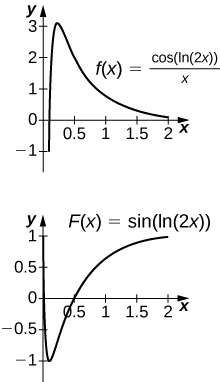 The antiderivative is [latex]y= \sin (\text{ln}(2x)).[/latex] Since the antiderivative is not continuous at [latex]x=0,[/latex] one cannot find a value of C that would make [latex]y= \sin (\text{ln}(2x))-C[/latex] work as a definite integral.
 13. [T][latex]\int \frac{3{x}^{2}+2x+1}{\sqrt{{x}^{3}+{x}^{2}+x+4}}dx[/latex] over [latex]\left[-1,2\right][/latex]
14. [T][latex]\int \frac{ \sin x}{{ \cos }^{3}x}dx[/latex] over [latex]\left[-\frac{\pi }{3},\frac{\pi }{3}\right][/latex]
Answer:
![Two graphs. The first is the function f(x) = sin(x) / cos(x)^3 over [-5pi/16, 5pi/16]. It is an increasing concave down function for values less than zero and an increasing concave up function for values greater than zero. The second is the fuction f(x) = ½ sec(x)^2 over the same interval. It is a wide, concave up curve which decreases for values less than zero and increases for values greater than zero.](https://s3-us-west-2.amazonaws.com/courses-images/wp-content/uploads/sites/2332/2018/01/11204239/CNX_Calc_Figure_05_05_206.jpg) The antiderivative is [latex]y=\frac{1}{2}\phantom{\rule{0.05em}{0ex}}{ \sec }^{2}x.[/latex] You should take [latex]C=-2[/latex] so that [latex]F(-\frac{\pi }{3})=0.[/latex]
The antiderivative is [latex]y=\frac{1}{2}\phantom{\rule{0.05em}{0ex}}{ \sec }^{2}x.[/latex] You should take [latex]C=-2[/latex] so that [latex]F(-\frac{\pi }{3})=0.[/latex]15. [T][latex]\int (x+2){e}^{\text{−}{x}^{2}-4x+3}dx[/latex] over [latex]\left[-5,1\right][/latex]
16. [T][latex]\int 3{x}^{2}\sqrt{2{x}^{3}+1}dx[/latex] over [latex]\left[0,1\right][/latex]
Answer:
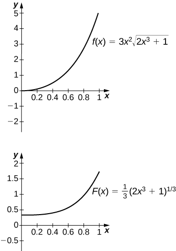 The antiderivative is [latex]y=\frac{1}{3}{(2{x}^{3}+1)}^{3\text{/}2}.[/latex] One should take [latex]C=-\frac{1}{3}.[/latex]
 17. If [latex]h(a)=h(b)[/latex] in [latex]{\int }_{a}^{b}g\text{‘}(h(x))h(x)dx,[/latex] what can you say about the value of the integral?
18. Is the substitution [latex]u=1-{x}^{2}[/latex] in the definite integral [latex]{\int }_{0}^{2}\frac{x}{1-{x}^{2}}dx[/latex] okay? If not, why not?
Answer:
No, because the integrand is discontinuous at [latex]x=1.[/latex]
In the following exercises, use a change of variables to show that each definite integral is equal to zero.
19. [latex]{\int }_{0}^{\pi }{ \cos }^{2}(2\theta ) \sin (2\theta )d\theta [/latex]
20. [latex]{\int }_{0}^{\sqrt{\pi }}t \cos ({t}^{2}) \sin ({t}^{2})dt[/latex]
Answer:
[latex]u= \sin ({t}^{2});[/latex] the integral becomes [latex]\frac{1}{2}{\int }_{0}^{0}udu.[/latex]
21. [latex]{\int }_{0}^{1}(1-2t)dt[/latex]
22. [latex]{\int }_{0}^{1}\frac{1-2t}{(1+{(t-\frac{1}{2})}^{2})}dt[/latex]
Answer:
[latex]u=(1+{(t-\frac{1}{2})}^{2});[/latex] the integral becomes [latex]\text{−}{\int }_{5\text{/}4}^{5\text{/}4}\frac{1}{u}du.[/latex]
23. [latex]{\int }_{0}^{\pi } \sin ({(t-\frac{\pi }{2})}^{3}) \cos (t-\frac{\pi }{2})dt[/latex]
24. [latex]{\int }_{0}^{2}(1-t) \cos (\pi t)dt[/latex]
Answer:
[latex]u=1-t;[/latex] the integral becomes
[latex-display]\begin{array}{l}{\int }_{1}^{-1}u \cos (\pi (1-u))du\hfill \\ ={\int }_{1}^{-1}u\left[ \cos \pi \cos u- \sin \pi \sin u\right]du\hfill \\ =\text{−}{\int }_{1}^{-1}u \cos udu\hfill \\ ={\int }_{-1}^{1}u \cos udu=0\hfill \end{array}[/latex-display] since the integrand is odd.25. [latex]{\int }_{\pi \text{/}4}^{3\pi \text{/}4}{ \sin }^{2}t \cos tdt[/latex]
26. Show that the average value of [latex]f(x)[/latex] over an interval [latex]\left[a,b\right][/latex] is the same as the average value of [latex]f(cx)[/latex] over the interval [latex]\left[\frac{a}{c},\frac{b}{c}\right][/latex] for [latex]c>0.[/latex]
Answer:
Setting [latex]u=cx[/latex] and [latex]du=cdx[/latex] gets you [latex]\frac{1}{\frac{b}{c}-\frac{a}{c}}{\int }_{a\text{/}c}^{b\text{/}c}f(cx)dx=\frac{c}{b-a}{\int }_{u=a}^{u=b}f(u)\frac{du}{c}=\frac{1}{b-a}{\int }_{a}^{b}f(u)du.[/latex]
27. Find the area under the graph of [latex]f(t)=\frac{t}{{(1+{t}^{2})}^{a}}[/latex] between [latex]t=0[/latex] and [latex]t=x[/latex] where [latex]a>0[/latex] and [latex]a\ne 1[/latex] is fixed, and evaluate the limit as [latex]x\to \infty .[/latex]
28. Find the area under the graph of [latex]g(t)=\frac{t}{{(1-{t}^{2})}^{a}}[/latex] between [latex]t=0[/latex] and [latex]t=x,[/latex] where [latex]0<x<1[/latex] and [latex]a>0[/latex] is fixed. Evaluate the limit as [latex]x\to 1.[/latex]
Answer:
[latex]{\int }_{0}^{x}g(t)dt=\frac{1}{2}{\int }_{u=1-{x}^{2}}^{1}\frac{du}{{u}^{a}}=\frac{1}{2(1-a)}{u}^{1-a}{|}_{u=1-{x}^{2}}^{1}=\frac{1}{2(1-a)}(1-{(1-{x}^{2})}^{1-a}).[/latex] As [latex]x\to 1[/latex] the limit is [latex]\frac{1}{2(1-a)}[/latex] if [latex]a<1,[/latex] and the limit diverges to +∞ if [latex]a>1.[/latex]
29. The area of a semicircle of radius 1 can be expressed as [latex]{\int }_{-1}^{1}\sqrt{1-{x}^{2}}dx.[/latex] Use the substitution [latex]x= \cos t[/latex] to express the area of a semicircle as the integral of a trigonometric function. You do not need to compute the integral.
30. The area of the top half of an ellipse with a major axis that is the [latex]x[/latex]-axis from [latex]x=-1[/latex] to [latex]a[/latex] and with a minor axis that is the [latex]y[/latex]-axis from [latex]y=\text{−}b[/latex] to [latex]b[/latex] can be written as [latex]{\int }_{\text{−}a}^{a}b\sqrt{1-\frac{{x}^{2}}{{a}^{2}}}dx.[/latex] Use the substitution [latex]x=a \cos t[/latex] to express this area in terms of an integral of a trigonometric function. You do not need to compute the integral.
Answer:
[latex]{\int }_{t=\pi }^{0}b\sqrt{1-{ \cos }^{2}t}×(\text{−}a \sin t)dt={\int }_{t=0}^{\pi }ab{ \sin }^{2}tdt[/latex]
31. [T] The following graph is of a function of the form [latex]f(t)=a \sin (nt)+b \sin (mt).[/latex] Estimate the coefficients [latex]a[/latex] and [latex]b[/latex], and the frequency parameters [latex]n[/latex] and [latex]m[/latex]. Use these estimates to approximate [latex]{\int }_{0}^{\pi }f(t)dt.[/latex]
![A graph of a function of the given form over [0, 2pi], which has six turning points. They are located at just before pi/4, just after pi/2, between 3pi/4 and pi, between pi and 5pi/4, just before 3pi/2, and just after 7pi/4 at about 3, -2, 1, -1, 2, and -3. It begins at the origin and ends at (2pi, 0). It crosses the x axis between pi/4 and pi/2, just before 3pi/4, pi, just after 5pi/4, and between 3pi/2 and 4pi/4.](https://s3-us-west-2.amazonaws.com/courses-images/wp-content/uploads/sites/2332/2018/01/11204247/CNX_Calc_Figure_05_05_201.jpg)
32. [T] The following graph is of a function of the form [latex]f(x)=a \cos (nt)+b \cos (mt).[/latex] Estimate the coefficients [latex]a[/latex] and [latex]b[/latex] and the frequency parameters [latex]n[/latex] and [latex]m[/latex]. Use these estimates to approximate [latex]{\int }_{0}^{\pi }f(t)dt.[/latex]
![The graph of a function of the given form over [0, 2pi]. It begins at (0,1) and ends at (2pi, 1). It has five turning points, located just after pi/4, between pi/2 and 3pi/4, pi, between 5pi/4 and 3pi/2, and just before 7pi/4 at about -1.5, 2.5, -3, 2.5, and -1. It crosses the x axis between 0 and pi/4, just before pi/2, just after 3pi/4, just before 5pi/4, just after 3pi/2, and between 7pi/4 and 2pi.](https://s3-us-west-2.amazonaws.com/courses-images/wp-content/uploads/sites/2332/2018/01/11204249/CNX_Calc_Figure_05_05_202.jpg)
Answer:
[latex]f(t)=2 \cos (3t)- \cos (2t);{\int }_{0}^{\pi \text{/}2}(2 \cos (3t)- \cos (2t))=-\frac{2}{3}[/latex]
33. [latex]{\int }_{0}^{\pi \text{/}4} \tan xdx[/latex]
34. [latex]{\int }_{0}^{\pi \text{/}3}\frac{ \sin x- \cos x}{ \sin x+ \cos x}dx[/latex]
Answer:
[latex]\text{ln}(\sqrt{3}-1)[/latex]
35. [latex]{\int }_{\pi \text{/}6}^{\pi \text{/}2} \csc xdx[/latex]
Answer:
[latex]\frac{1}{2}\text{ln}\frac{3}{2}[/latex]
In the following exercises, does the right-endpoint approximation overestimate or underestimate the exact area? Calculate the right endpoint estimate R50 and solve for the exact area.
37. [T][latex]y={e}^{x}[/latex] over [latex]\left[0,1\right][/latex]
38. [T][latex]y={e}^{\text{−}x}[/latex] over [latex]\left[0,1\right][/latex]
Answer:
Exact solution: [latex]\frac{e-1}{e},{R}_{50}=0.6258.[/latex] Since [latex]f[/latex] is decreasing, the right endpoint estimate underestimates the area.
39. [T][latex]y=\text{ln}(x)[/latex] over [latex]\left[1,2\right][/latex]
40. [T][latex]y=\frac{x+1}{{x}^{2}+2x+6}[/latex] over [latex]\left[0,1\right][/latex]
Answer:
Exact solution: [latex]\frac{2\text{ln}(3)-\text{ln}(6)}{2},{R}_{50}=0.2033.[/latex] Since [latex]f[/latex] is increasing, the right endpoint estimate overestimates the area.
41. [T][latex]y={2}^{x}[/latex] over [latex]\left[-1,0\right][/latex]
42. [T][latex]y=\text{−}{2}^{\text{−}x}[/latex] over [latex]\left[0,1\right][/latex]
Answer:
Exact solution: [latex]-\frac{1}{\text{ln}(4)},{R}_{50}=-0.7164.[/latex] Since [latex]f[/latex] is increasing, the right endpoint estimate overestimates the area (the actual area is a larger negative number).
In the following exercises, [latex]f(x)\ge 0[/latex] for [latex]a\le x\le b.[/latex] Find the area under the graph of [latex]f(x)[/latex] between the given values [latex]a[/latex] and [latex]b[/latex] by integrating.
43. [latex]f(x)=\frac{{\text{log}}_{10}(x)}{x};a=10,b=100[/latex]
44. [latex]f(x)=\frac{{\text{log}}_{2}(x)}{x};a=32,b=64[/latex]
Answer:
[latex]\frac{11}{2}\text{ln}2[/latex]
45. [latex]f(x)={2}^{\text{−}x};a=1,b=2[/latex]
46. [latex]f(x)={2}^{\text{−}x};a=3,b=4[/latex]
Answer:
[latex]\frac{1}{\text{ln}(65,536)}[/latex]
47. Find the area under the graph of the function [latex]f(x)=x{e}^{\text{−}{x}^{2}}[/latex] between [latex]x=0[/latex] and [latex]x=5.[/latex]
48. Compute the integral of [latex]f(x)=x{e}^{\text{−}{x}^{2}}[/latex] and find the smallest value of N such that the area under the graph [latex]f(x)=x{e}^{\text{−}{x}^{2}}[/latex] between [latex]x=N[/latex] and [latex]x=N+10[/latex] is, at most, 0.01.
Answer: [latex]{\int }_{N}^{N+1}x{e}^{\text{−}{x}^{2}}dx=\frac{1}{2}({e}^{\text{−}{N}^{2}}-{e}^{\text{−}{(N+1)}^{2}}).[/latex] The quantity is less than 0.01 when [latex]N=2.[/latex]
49. Find the limit, as N tends to infinity, of the area under the graph of [latex]f(x)=x{e}^{\text{−}{x}^{2}}[/latex] between [latex]x=0[/latex] and [latex]x=5.[/latex]
50. Show that [latex]{\int }_{a}^{b}\frac{dt}{t}={\int }_{1\text{/}b}^{1\text{/}a}\frac{dt}{t}[/latex] when [latex]0<a\le b.[/latex]
Answer:
[latex]{\int }_{a}^{b}\frac{dx}{x}=\text{ln}(b)-\text{ln}(a)=\text{ln}(\frac{1}{a})-\text{ln}(\frac{1}{b})={\int }_{1\text{/}b}^{1\text{/}a}\frac{dx}{x}[/latex]
51. Suppose that [latex]f(x)>0[/latex] for all [latex]x[/latex] and that [latex]f[/latex] and [latex]g[/latex] are differentiable. Use the identity [latex]{f}^{g}={e}^{g\text{ln}f}[/latex] and the chain rule to find the derivative of [latex]{f}^{g}.[/latex]
52. Use the previous exercise to find the antiderivative of [latex]h(x)={x}^{x}(1+\text{ln}x)[/latex] and evaluate [latex]{\int }_{2}^{3}{x}^{x}(1+\text{ln}x)dx.[/latex]
Answer:
23
53. Show that if [latex]c>0,[/latex] then the integral of [latex]1\text{/}x[/latex] from ac to bc [latex](0<a<b)[/latex] is the same as the integral of [latex]1\text{/}x[/latex] from [latex]a[/latex] to [latex]b[/latex].
The following exercises are intended to derive the fundamental properties of the natural log starting from the Definition/em> [latex]\text{ln}(x)={\int }_{1}^{x}\frac{dt}{t},[/latex] using properties of the definite integral and making no further assumptions.
54. Use the identity [latex]\text{ln}(x)={\int }_{1}^{x}\frac{dt}{t}[/latex] to derive the identity [latex]\text{ln}(\frac{1}{x})=\text{−}\text{ln}x.[/latex]
Answer:
We may assume that [latex]x>1,\text{so}\frac{1}{x}<1.[/latex] Then, [latex]{\int }_{1}^{1\text{/}x}\frac{dt}{t}.[/latex] Now make the substitution [latex]u=\frac{1}{t},[/latex] so [latex]du=-\frac{dt}{{t}^{2}}[/latex] and [latex]\frac{du}{u}=-\frac{dt}{t},[/latex] and change endpoints: [latex]{\int }_{1}^{1\text{/}x}\frac{dt}{t}=\text{−}{\int }_{1}^{x}\frac{du}{u}=\text{−}\text{ln}x.[/latex]
56. Use the identity [latex]\text{ln}x={\int }_{1}^{x}\frac{dt}{x}[/latex] to show that [latex]\text{ln}(x)[/latex] is an increasing function of [latex]x[/latex] on [latex][0,\infty )[/latex] and use the previous exercises to show that the range of [latex]\text{ln}(x)[/latex] is [latex](\text{−}\infty ,\infty ).[/latex] Without any further assumptions, conclude that [latex]\text{ln}(x)[/latex] has an inverse function defined on [latex](\text{−}\infty ,\infty ).[/latex]
57. Pretend, for the moment, that we do not know that [latex]{e}^{x}[/latex] is the inverse function of [latex]\text{ln}(x),[/latex] but keep in mind that [latex]\text{ln}(x)[/latex] has an inverse function defined on [latex](\text{−}\infty ,\infty ).[/latex] Call it E. Use the identity [latex]\text{ln}xy=\text{ln}x+\text{ln}y[/latex] to deduce that [latex]E(a+b)=E(a)E(b)[/latex] for any real numbers [latex]a[/latex], [latex]b[/latex].
58. Pretend, for the moment, that we do not know that [latex]{e}^{x}[/latex] is the inverse function of [latex]\text{ln}x,[/latex] but keep in mind that [latex]\text{ln}x[/latex] has an inverse function defined on [latex](\text{−}\infty ,\infty ).[/latex] Call it E. Show that [latex]E\text{'}(t)=E(t).[/latex]
Answer:
[latex]x=E(\text{ln}(x)).[/latex] Then, [latex]1=\frac{E\text{'}(\text{ln}x)}{x}\text{or}x=E\text{'}(\text{ln}x).[/latex] Since any number [latex]t[/latex] can be written [latex]t=\text{ln}x[/latex] for some [latex]x[/latex], and for such [latex]t[/latex] we have [latex]x=E(t),[/latex] it follows that for any [latex]t,E\text{'}(t)=E(t).[/latex]
59. The sine integral, defined as [latex]S(x)={\int }_{0}^{x}\frac{ \sin t}{t}dt[/latex] is an important quantity in engineering. Although it does not have a simple closed formula, it is possible to estimate its behavior for large [latex]x[/latex]. Show that for [latex]k\ge 1,|S(2\pi k)-S(2\pi (k+1))|\le \frac{1}{k(2k+1)\pi }.[/latex](Hint: [latex]\sin (t+\pi )=\text{−} \sin t[/latex])
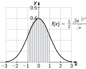
60. [T] The normal distribution in probability is given by [latex]p(x)=\frac{1}{\sigma \sqrt{2\pi }}{e}^{\text{−}{(x-\mu )}^{2}\text{/}2{\sigma }^{2}},[/latex] where σ is the standard deviation and μ is the average. The standard normal distribution in probability, [latex]{p}_{s},[/latex] corresponds to [latex]\mu =0\text{ and }\sigma =1.[/latex] Compute the left endpoint estimates [latex]{R}_{10}\text{ and }{R}_{100}[/latex] of [latex]{\int }_{-1}^{1}\frac{1}{\sqrt{2\pi }}{e}^{\text{−}{x}^{2\text{/}2}}dx.[/latex]
Answer:
[latex]{R}_{10}=0.6811,{R}_{100}=0.6827[/latex]
61. [T] Compute the right endpoint estimates [latex]{R}_{50}\text{ and }{R}_{100}[/latex] of [latex]{\int }_{-3}^{5}\frac{1}{2\sqrt{2\pi }}{e}^{\text{−}{(x-1)}^{2}\text{/}8}.[/latex]
In the following exercises, evaluate each integral in terms of an inverse trigonometric function.
62. [latex]{\int }_{0}^{\sqrt{3}\text{/}2}\frac{dx}{\sqrt{1-{x}^{2}}}[/latex]
Answer:
[latex]{ \sin }^{-1}x{|}_{0}^{\sqrt{3}\text{/}2}=\frac{\pi }{3}[/latex]
63. [latex]{\int }_{-1\text{/}2}^{1\text{/}2}\frac{dx}{\sqrt{1-{x}^{2}}}[/latex]
64. [latex]{\int }_{\sqrt{3}}^{1}\frac{dx}{\sqrt{1+{x}^{2}}}[/latex]
Answer:
[latex]{ \tan }^{-1}x{|}_{\sqrt{3}}^{1}=-\frac{\pi }{12}[/latex]
65. [latex]{\int }_{1\text{/}\sqrt{3}}^{\sqrt{3}}\frac{dx}{1+{x}^{2}}[/latex]
66. [latex]{\int }_{1}^{\sqrt{2}}\frac{dx}{|x|\sqrt{{x}^{2}-1}}[/latex]
Answer:
[latex]{ \sec }^{-1}x{|}_{1}^{\sqrt{2}}=\frac{\pi }{4}[/latex]
67. [latex]{\int }_{1}^{2\text{/}\sqrt{3}}\frac{dx}{|x|\sqrt{{x}^{2}-1}}[/latex]
68. Explain what is wrong with the following integral: [latex]{\int }_{1}^{2}\frac{dt}{\sqrt{1-{t}^{2}}}.[/latex]
Answer:
[latex]\sqrt{1-{t}^{2}}[/latex] is not defined as a real number when [latex]t>1.[/latex]
69. Explain what is wrong with the following integral: [latex]{\int }_{-1}^{1}\frac{dt}{|t|\sqrt{{t}^{2}-1}}.[/latex]
70. [T][latex]\int \frac{1}{\sqrt{9-{x}^{2}}}dx[/latex] over [latex]\left[-3,3\right][/latex]
Answer:  The antiderivative is [latex]{ \sin }^{-1}(\frac{x}{3})+C.[/latex] Taking [latex]C=\frac{\pi }{2}[/latex] recovers the definite integral.
71. [T][latex]\int \frac{9}{9+{x}^{2}}dx[/latex] over [latex]\left[-6,6\right][/latex]
Answer: ![Two graphs. The first shows the function f(x) = cos(x) / (4 + sin(x)^2). It is an oscillating function over [-6, 6] with turning points at roughly (-3, -2.5), (0, .25), and (3, -2.5), where (0,.25) is a local max and the others are local mins. The second shows the function F(x) = .5 * arctan(.5*sin(x)), which also oscillates over [-6,6]. It has turning points at roughly (-4.5, .25), (-1.5, -.25), (1.5, .25), and (4.5, -.25).](https://s3-us-west-2.amazonaws.com/courses-images/wp-content/uploads/sites/2332/2018/01/11204305/CNX_Calc_Figure_05_07_203.jpg) The antiderivative is [latex]\frac{1}{2}\phantom{\rule{0.05em}{0ex}}{ \tan }^{-1}(\frac{ \sin x}{2})+C.[/latex] Taking [latex]C=\frac{1}{2}\phantom{\rule{0.05em}{0ex}}{ \tan }^{-1}(\frac{ \sin (6)}{2})[/latex] recovers the definite integral.
The antiderivative is [latex]\frac{1}{2}\phantom{\rule{0.05em}{0ex}}{ \tan }^{-1}(\frac{ \sin x}{2})+C.[/latex] Taking [latex]C=\frac{1}{2}\phantom{\rule{0.05em}{0ex}}{ \tan }^{-1}(\frac{ \sin (6)}{2})[/latex] recovers the definite integral.
73. [T][latex]\int \frac{{e}^{x}}{1+{e}^{2x}}dx[/latex] over [latex]\left[-6,6\right][/latex]
74. [T][latex]\int \frac{1}{x\sqrt{{x}^{2}-4}}dx[/latex] over [latex]\left[2,6\right][/latex]
Answer:  The antiderivative is [latex]\frac{1}{2}\phantom{\rule{0.05em}{0ex}}{ \sec }^{-1}(\frac{x}{2})+C.[/latex] Taking [latex]C=0[/latex] recovers the definite integral over [latex]\left[2,6\right].[/latex]
75. [T][latex]\int \frac{1}{(2x+2)\sqrt{x}}dx[/latex] over [latex]\left[0,6\right][/latex]
76. [T][latex]\int \frac{( \sin x+x \cos x)}{1+{x}^{2}{ \sin }^{2}x}dx[/latex] over [latex]\left[-6,6\right][/latex]
![The graph of f(x) = arctan(x sin(x)) over [-6,6]. It has five turning points at roughly (-5, -1.5), (-2,1), (0,0), (2,1), and (5,-1.5).](https://s3-us-west-2.amazonaws.com/courses-images/wp-content/uploads/sites/2332/2018/01/11204310/CNX_Calc_Figure_05_07_207.jpg) The general antiderivative is [latex]{ \tan }^{-1}(x \sin x)+C.[/latex] Taking [latex]C=\text{−}{ \tan }^{-1}(6 \sin (6))[/latex] recovers the definite integral.
The general antiderivative is [latex]{ \tan }^{-1}(x \sin x)+C.[/latex] Taking [latex]C=\text{−}{ \tan }^{-1}(6 \sin (6))[/latex] recovers the definite integral.
77. [T][latex]\int \frac{2{e}^{-2x}}{\sqrt{1-{e}^{-4x}}}dx[/latex] over [latex]\left[0,2\right][/latex]
78. [T][latex]\int \frac{1}{x+x{\text{ln}}^{2}x}[/latex] over [latex]\left[0,2\right][/latex]
![A graph of the function f(x) = arctan(ln(x)) over (0, 2]. It is an increasing curve with x-intercept at (1,0).](https://s3-us-west-2.amazonaws.com/courses-images/wp-content/uploads/sites/2332/2018/01/11204313/CNX_Calc_Figure_05_07_209.jpg) The general antiderivative is [latex]{ \tan }^{-1}(\text{ln}x)+C.[/latex] Taking [latex]C=\frac{\pi }{2}={ \tan }^{-1}\infty [/latex] recovers the definite integral.
The general antiderivative is [latex]{ \tan }^{-1}(\text{ln}x)+C.[/latex] Taking [latex]C=\frac{\pi }{2}={ \tan }^{-1}\infty [/latex] recovers the definite integral.
79. [T][latex]\int \frac{{ \sin }^{-1}x}{\sqrt{1-{x}^{2}}}[/latex] over [latex]\left[-1,1\right][/latex]
In the following exercises, compute each definite integral.
80. [latex]{\int }_{0}^{1\text{/}2}\frac{ \tan ({ \sin }^{-1}t)}{\sqrt{1-{t}^{2}}}dt[/latex]
Answer: [latex]\frac{1}{2}\text{ln}(\frac{4}{3})[/latex]
81. [latex]{\int }_{1\text{/}4}^{1\text{/}2}\frac{ \tan ({ \cos }^{-1}t)}{\sqrt{1-{t}^{2}}}dt[/latex]
Answer:
[latex]1-\frac{2}{\sqrt{5}}[/latex]
83. [latex]{\int }_{0}^{1\text{/}2}\frac{ \cos ({ \tan }^{-1}t)}{1+{t}^{2}}dt[/latex]
84. For [latex]A>0,[/latex] compute [latex]I(A)={\int }_{\text{−}A}^{A}\frac{dt}{1+{t}^{2}}[/latex] and evaluate [latex]\underset{a\to \infty }{\text{lim}}I(A),[/latex] the area under the graph of [latex]\frac{1}{1+{t}^{2}}[/latex] on [latex]\left[\text{−}\infty ,\infty \right].[/latex]
Answer:
[latex]2{ \tan }^{-1}(A)\to \pi [/latex] as [latex]A\to \infty [/latex]
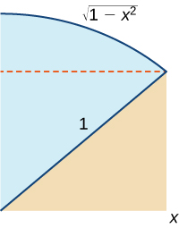
85. Use the following graph to prove that [latex]{\int }_{0}^{x}\sqrt{1-{t}^{2}}dt=\frac{1}{2}x\sqrt{1-{x}^{2}}+\frac{1}{2}\phantom{\rule{0.05em}{0ex}}{ \sin }^{-1}x.[/latex]
Glossary
- change of variables
- the substitution of a variable, such as [latex]u[/latex], for an expression in the integrand
- integration by substitution
- a technique for integration that allows integration of functions that are the result of a chain-rule derivative
Licenses & Attributions
CC licensed content, Shared previously
- Calculus I. Provided by: OpenStax Located at: https://openstax.org/books/calculus-volume-1/pages/1-introduction. License: CC BY-NC-SA: Attribution-NonCommercial-ShareAlike. License terms: Download for free at http://cnx.org/contents/[email protected].

Hint
Let [latex]u=2x.[/latex]