One-Sided Limits
Learning Objectives
- Define one-sided limits and provide examples.
- Explain the relationship between one-sided and two-sided limits.
- Define a vertical asymptote.
One-Sided Limits
Sometimes indicating that the limit of a function fails to exist at a point does not provide us with enough information about the behavior of the function at that particular point. To see this, we now revisit the function [latex]g(x)=|x-2|/(x-2)[/latex] introduced at the beginning of the section (see (Figure)(b)). As we pick values of [latex]x[/latex] close to 2, [latex]g(x)[/latex] does not approach a single value, so the limit as [latex]x[/latex] approaches 2 does not exist—that is, [latex]\underset{x\to 2}{\lim}g(x)[/latex] DNE. However, this statement alone does not give us a complete picture of the behavior of the function around the [latex]x[/latex]-value 2. To provide a more accurate description, we introduce the idea of a one-sided limit. For all values to the left of 2 (or the negative side of 2), [latex]g(x)=-1[/latex]. Thus, as [latex]x[/latex] approaches 2 from the left, [latex]g(x)[/latex] approaches −1. Mathematically, we say that the limit as [latex]x[/latex] approaches 2 from the left is −1. Symbolically, we express this idea as
Similarly, as [latex]x[/latex] approaches 2 from the right (or from the positive side), [latex]g(x)[/latex] approaches 1. Symbolically, we express this idea as
We can now present an informal definition of one-sided limits.
Definition
We define two types of one-sided limits.
Limit from the left: Let [latex]f(x)[/latex] be a function defined at all values in an open interval of the form z, and let [latex]L[/latex] be a real number. If the values of the function [latex]f(x)[/latex] approach the real number [latex]L[/latex] as the values of [latex]x[/latex] (where [latex]x<a[/latex]) approach the number [latex]a[/latex], then we say that [latex]L[/latex] is the limit of [latex]f(x)[/latex] as [latex]x[/latex] approaches a from the left. Symbolically, we express this idea as
Limit from the right: Let [latex]f(x)[/latex] be a function defined at all values in an open interval of the form [latex](a,c)[/latex], and let [latex]L[/latex] be a real number. If the values of the function [latex]f(x)[/latex] approach the real number [latex]L[/latex] as the values of [latex]x[/latex] (where [latex]x>a[/latex]) approach the number [latex]a[/latex], then we say that [latex]L[/latex] is the limit of [latex]f(x)[/latex] as [latex]x[/latex] approaches [latex]a[/latex] from the right. Symbolically, we express this idea as
Evaluating One-Sided Limits
For the function [latex]f(x)=\begin{cases} x+1, & \text{if} \, x < 2 \\ x^2-4, & \text{if} \, x \ge 2 \end{cases}[/latex], evaluate each of the following limits.
- [latex]\underset{x\to 2^-}{\lim}f(x)[/latex]
- [latex]\underset{x\to 2^+}{\lim}f(x)[/latex]
Answer:
We can use tables of functional values again (Figure). Observe that for values of [latex]x[/latex] less than 2, we use [latex]f(x)=x+1[/latex] and for values of [latex]x[/latex] greater than 2, we use [latex]f(x)=x^2-4[/latex].
| [latex]x[/latex] | [latex]f(x)=x+1[/latex] | [latex]x[/latex] | [latex]f(x)=x^2-4[/latex] | |
|---|---|---|---|---|
| 1.9 | 2.9 | 2.1 | 0.41 | |
| 1.99 | 2.99 | 2.01 | 0.0401 | |
| 1.999 | 2.999 | 2.001 | 0.004001 | |
| 1.9999 | 2.9999 | 2.0001 | 0.00040001 | |
| 1.99999 | 2.99999 | 2.00001 | 0.0000400001 |
Based on this table, we can conclude that a. [latex]\underset{x\to 2^-}{\lim}f(x)=3[/latex] and b. [latex]\underset{x\to 2^+}{\lim}f(x)=0[/latex]. Therefore, the (two-sided) limit of [latex]f(x)[/latex] does not exist at [latex]x=2[/latex]. (Figure) shows a graph of [latex]f(x)[/latex] and reinforces our conclusion about these limits.
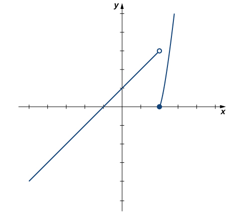 Figure 7. The graph of [latex]f(x)=\begin{cases} x+1, & \text{if} \, x < 2 \\ x^2-4, & \text{if} \, x \ge 2 \end{cases}[/latex] has a break at [latex]x=2[/latex].
Use a table of functional values to estimate the following limits, if possible.
- [latex]\underset{x\to 2^-}{\lim}\frac{|x^2-4|}{x-2}[/latex]
- [latex]\underset{x\to 2^+}{\lim}\frac{|x^2-4|}{x-2}[/latex]
Answer:
a. [latex]\underset{x\to 2^-}{\lim}\frac{|x^2-4|}{x-2}=-4[/latex]; b. [latex]\underset{x\to 2^+}{\lim}\frac{|x^2-4|}{x-2}=4[/latex]
Simple modifications in the limit laws allow us to apply them to one-sided limits. For example, to apply the limit laws to a limit of the form [latex]\underset{x\to a^-}{\lim}h(x)[/latex], we require the function [latex]h(x)[/latex] to be defined over an open interval of the form [latex](b,a)[/latex]; for a limit of the form [latex]\underset{x\to a^+}{\lim}h(x)[/latex], we require the function [latex]h(x)[/latex] to be defined over an open interval of the form [latex](a,c)[/latex]. (Figure) illustrates this point.
Evaluating a One-Sided Limit Using the Limit Laws
Evaluate each of the following limits, if possible.
- [latex]\underset{x\to 3^-}{\lim}\sqrt{x-3}[/latex]
- [latex]\underset{x\to 3^+}{\lim}\sqrt{x-3}[/latex]
Answer:
(Figure) illustrates the function [latex]f(x)=\sqrt{x-3}[/latex] and aids in our understanding of these limits.
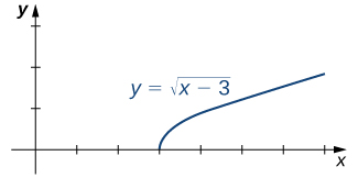 Figure 2. The graph shows the function [latex]f(x)=\sqrt{x-3}[/latex].
- The function [latex]f(x)=\sqrt{x-3}[/latex] is defined over the interval [latex][3,+\infty)[/latex]. Since this function is not defined to the left of 3, we cannot apply the limit laws to compute [latex]\underset{x\to 3^-}{\lim}\sqrt{x-3}[/latex]. In fact, since [latex]f(x)=\sqrt{x-3}[/latex] is undefined to the left of 3, [latex]\underset{x\to 3^-}{\lim}\sqrt{x-3}[/latex] does not exist.
- Since [latex]f(x)=\sqrt{x-3}[/latex] is defined to the right of 3, the limit laws do apply to [latex]\underset{x\to 3^+}{\lim}\sqrt{x-3}[/latex]. By applying these limit laws we obtain [latex]\underset{x\to 3^+}{\lim}\sqrt{x-3}=0[/latex].
In (Figure) we look at one-sided limits of a piecewise-defined function and use these limits to draw a conclusion about a two-sided limit of the same function.
Evaluating a Two-Sided Limit Using the Limit Laws
For [latex]f(x)=\begin{cases} 4x-3 & \text{if} \, x<2 \\ (x-3)^2 & \text{if} \, x \ge 2 \end{cases}[/latex] evaluate each of the following limits:
- [latex]\underset{x\to 2^-}{\lim}f(x)[/latex]
- [latex]\underset{x\to 2^+}{\lim}f(x)[/latex]
- [latex]\underset{x\to 2}{\lim}f(x)[/latex]
Answer:
(Figure) illustrates the function [latex]f(x)[/latex] and aids in our understanding of these limits.
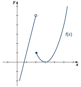 Figure 3. This graph shows the function [latex]f(x)[/latex].
- Since [latex]f(x)=4x-3[/latex] for all [latex]x[/latex] in [latex](−\infty,2)[/latex], replace [latex]f(x)[/latex] in the limit with [latex]4x-3[/latex] and apply the limit laws:
[latex]\underset{x\to 2^-}{\lim}f(x)=\underset{x\to 2^-}{\lim}(4x-3)=5[/latex].
- Since [latex]f(x)=(x-3)^2[/latex] for all [latex]x[/latex] in [latex](2,+\infty)[/latex], replace [latex]f(x)[/latex] in the limit with [latex](x-3)^2[/latex] and apply the limit laws:
[latex]\underset{x\to 2^+}{\lim}f(x)=\underset{x\to 2^-}{\lim}(x-3)^2=1[/latex].
- Since [latex]\underset{x\to 2^-}{\lim}f(x)=5[/latex] and [latex]\underset{x\to 2^+}{\lim}f(x)=1[/latex], we conclude that [latex]\underset{x\to 2}{\lim}f(x)[/latex] does not exist.
Graph [latex]f(x)=\begin{cases} -x-2 & \text{if} \, x<-1 \\ 2 & \text{if} \, x = -1 \\ x^3 & \text{if} \, x > -1 \end{cases}[/latex] and evaluate [latex]\underset{x\to -1^-}{\lim}f(x)[/latex].
Answer: 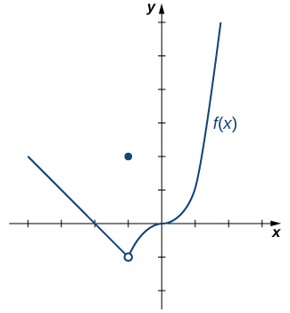 [latex]\underset{x\to -1^-}{\lim}f(x)=-1[/latex]
Hint
Use the method in (Figure) to evaluate the limit.
evaluating one-sided limits from a graph
Use the graph of [latex]f(x)[/latex] in (Figure) to determine each of the following values:
- [latex]\underset{x\to -4^-}{\lim}f(x); \, \underset{x\to -4^+}{\lim}f(x); \, \underset{x\to -4}{\lim}f(x); \, f(-4)[/latex]
- [latex]\underset{x\to -2^-}{\lim}f(x); \, \underset{x\to -2^+}{\lim}f(x); \, \underset{x\to -2}{\lim}f(x); \, f(-2)[/latex]
- [latex]\underset{x\to 1^-}{\lim}f(x); \, \underset{x\to 1^+}{\lim}f(x); \, \underset{x\to 1}{\lim}f(x); \, f(1)[/latex]
![The graph of a function f(x) described by the above limits and values. There is a smooth curve for values below x=-2; at (-2, 3), there is an open circle. There is a smooth curve between (-2, 1] with a closed circle at (1,6). There is an open circle at (1,3), and a smooth curve stretching from there down asymptotically to negative infinity along x=3. The function also curves asymptotically along x=3 on the other side, also stretching to negative infinity. The function then changes concavity in the first quadrant around y=4.5 and continues up.](https://s3-us-west-2.amazonaws.com/courses-images/wp-content/uploads/sites/2332/2018/01/11202918/CNX_Calc_Figure_02_02_015.jpg) Figure 10. The graph shows [latex]f(x)[/latex].
Figure 10. The graph shows [latex]f(x)[/latex].Answer:
Using (Figure) and the graph for reference, we arrive at the following values:
- [latex]\underset{x\to -4^-}{\lim}f(x)=0; \, \underset{x\to -4^+}{\lim}f(x)=0; \, \underset{x\to -4}{\lim}f(x)=0; \, f(-4)=0[/latex]
- [latex]\underset{x\to -2^-}{\lim}f(x)=3; \, \underset{x\to -2^+}{\lim}f(x)=3; \, \underset{x\to -2}{\lim}f(x)=3; \, f(-2)[/latex] is undefined
- [latex]\underset{x\to 1^-}{\lim}f(x)=6; \, \underset{x\to 1^+}{\lim}f(x)=3; \, \underset{x\to 1}{\lim}f(x)=DNE[/latex]; [latex]f(1)=6[/latex]
We will now recall the Squeeze Theorem to prove two special limits. The first of these limits is [latex]\underset{\theta \to 0}{\lim} \sin \theta[/latex]. Consider the unit circle shown in (Figure). In the figure, we see that [latex] \sin \theta [/latex] is the [latex]y[/latex]-coordinate on the unit circle and it corresponds to the line segment shown in blue. The radian measure of angle θ is the length of the arc it subtends on the unit circle. Therefore, we see that for [latex]0<\theta <\frac{\pi }{2}, \, 0 < \sin \theta < \theta[/latex].
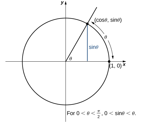 Figure 6. The sine function is shown as a line on the unit circle.
Because [latex]\underset{\theta \to 0^+}{\lim}0=0[/latex] and [latex]\underset{\theta \to 0^+}{\lim}\theta =0[/latex], by using the Squeeze Theorem we conclude that
To see that [latex]\underset{\theta \to 0^-}{\lim} \sin \theta =0[/latex] as well, observe that for [latex]-\frac{\pi }{2} < \theta <0, \, 0 < −\theta < \frac{\pi}{2}[/latex] and hence, [latex]0 < \sin(-\theta) < −\theta[/latex]. Consequently, [latex]0 < -\sin \theta < −\theta[/latex] It follows that [latex]0 > \sin \theta > \theta[/latex]. An application of the Squeeze Theorem produces the desired limit. Thus, since [latex]\underset{\theta \to 0^+}{\lim} \sin \theta =0[/latex] and [latex]\underset{\theta \to 0^-}{\lim} \sin \theta =0[/latex],
Next, using the identity [latex] \cos \theta =\sqrt{1-\sin^2 \theta}[/latex] for [latex]-\frac{\pi}{2}<\theta <\frac{\pi}{2}[/latex], we see that
We now take a look at a limit that plays an important role in later chapters—namely, [latex]\underset{\theta \to 0}{\lim}\frac{\sin \theta}{\theta}[/latex]. To evaluate this limit, we use the unit circle in (Figure). Notice that this figure adds one additional triangle to (Figure). We see that the length of the side opposite angle [latex]\theta[/latex] in this new triangle is [latex]\tan \theta[/latex]. Thus, we see that for [latex]0 < \theta < \frac{\pi}{2}, \, \sin \theta < \theta < \tan \theta[/latex].
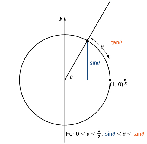 Figure 7. The sine and tangent functions are shown as lines on the unit circle.
By dividing by [latex]\sin \theta [/latex] in all parts of the inequality, we obtain
Equivalently, we have
Since [latex]\underset{\theta \to 0^+}{\lim}1=1=\underset{\theta \to 0^+}{\lim}\cos \theta[/latex], we conclude that [latex]\underset{\theta \to 0^+}{\lim}\frac{\sin \theta}{\theta}=1[/latex]. By applying a manipulation similar to that used in demonstrating that [latex]\underset{\theta \to 0^-}{\lim}\sin \theta =0[/latex], we can show that [latex]\underset{\theta \to 0^-}{\lim}\frac{\sin \theta}{\theta}=1[/latex]. Thus,
In (Figure) we use this limit to establish [latex]\underset{\theta \to 0}{\lim}\frac{1- \cos \theta}{\theta}=0[/latex]. This limit also proves useful in later chapters.
Evaluating an Important Trigonometric Limit
Evaluate [latex]\underset{\theta \to 0}{\lim}\frac{1- \cos \theta}{\theta}[/latex].
Answer:
In the first step, we multiply by the conjugate so that we can use a trigonometric identity to convert the cosine in the numerator to a sine:
Therefore,
Evaluate [latex]\underset{\theta \to 0}{\lim}\frac{1- \cos \theta}{\sin \theta}[/latex].
Answer:
0
Hint
Multiply numerator and denominator by [latex]1+ \cos \theta[/latex].
Special Trigonometric Limits
Summarizing our work from above we have two special limits: [latex]\underset{\theta \to 0}{\lim}\frac{\sin \theta}{\theta}=1[/latex] and [latex]\underset{\theta \to 0}{\lim}\frac{1- \cos \theta}{\theta}=0[/latex]Evaluating a Limit involving [latex]\frac{\sin \theta}{\theta}[/latex] and [latex]\frac{1-\cos\theta}{\theta}[/latex]
Evaluate [latex]\underset{\theta \to 0}{\lim}\frac{\sin 3\theta}{2\theta}[/latex].
Answer:
In the first step, we multiply by a power of one:
Therefore,
Evaluate [latex]\underset{\theta \to 0}{\lim}\frac{1- \cos 3\theta}{9\theta}[/latex].
Answer:
0
Hint
Divide the numerator and denominator by [latex]3[/latex].
Key Equations
- One-Sided Limits [latex-display]\underset{x\to a^-}{\lim}f(x)=L[/latex-display] [latex]\underset{x\to a^+}{\lim}f(x)=L[/latex]
- Important Limits [latex-display]\underset{\theta \to 0}{\lim}\frac{\sin \theta}{\theta}=1[/latex-display] [latex]\underset{\theta \to 0}{\lim}\frac{1- \cos \theta}{\theta}=0[/latex]
In the following exercises, set up a table of values to find the indicated limit. Round to eight digits.
1. [T] [latex]\underset{t\to 0^+}{\lim}\frac{\cos t}{t}[/latex]
| [latex]t[/latex] | [latex]\frac{\cos t}{t}[/latex] |
|---|---|
| 0.1 | a. |
| 0.01 | b. |
| 0.001 | c. |
| 0.0001 | d. |
2. [T] [latex]\underset{x\to 2^-}{\lim}\frac{1-\frac{2}{x}}{x^2-4}[/latex]
| [latex]x[/latex] | [latex]\frac{1-\frac{2}{x}}{x^2-4}[/latex] | [latex]x[/latex] | [latex]\frac{1-\frac{2}{x}}{x^2-4}[/latex] |
|---|---|---|---|
| 1.9 | a. | 2.1 | e. |
| 1.99 | b. | 2.01 | f. |
| 1.999 | c. | 2.001 | g. |
| 1.9999 | d. | 2.0001 | h. |
Answer:
a. 0.13495277; b. 0.12594300; c. 0.12509381; d. 0.12500938; e. 0.11614402; f. 0.12406794; g. 0.12490631; h. 0.12499063;
[latex-display]\underset{x\to 2^-}{\lim}\frac{1-\frac{2}{x}}{x^2-4}=0.1250=\frac{1}{8}[/latex-display]In the following exercises, set up a table of values and round to eight significant digits. Based on the table of values, make a guess about what the limit is. Then, use a calculator to graph the function and determine the limit. Was the conjecture correct? If not, why does the method of tables fail?
3. [T] [latex]\underset{\theta \to 0^-}{\lim}\sin (\frac{\pi }{\theta })[/latex]
| θ | [latex] \sin (\frac{\pi }{\theta })[/latex] | θ | [latex] \sin (\frac{\pi }{\theta })[/latex] |
|---|---|---|---|
| −0.1 | a. | 0.1 | e. |
| −0.01 | b. | 0.01 | f. |
| −0.001 | c. | 0.001 | g. |
| −0.0001 | d. | 0.0001 | h. |
4. [T] [latex]\underset{\alpha \to 0^+}{\lim}\frac{1}{\alpha } \cos (\frac{\pi }{\alpha })[/latex]
| [latex]a[/latex] | [latex]\frac{1}{\alpha } \cos (\frac{\pi }{\alpha })[/latex] |
|---|---|
| 0.1 | a. |
| 0.01 | b. |
| 0.001 | c. |
| 0.0001 | d. |
Answer:
a. −10.00000; b. −100.00000; c. −1000.0000; d. −10,000.000; Guess: [latex]\underset{\alpha \to 0^+}{\lim}\frac{1}{\alpha } \cos (\frac{\pi }{\alpha })=\infty[/latex], Actual: DNE
![A graph of the function (1/alpha) * cos (pi / alpha), which oscillates gently until the interval [-.2, .2], where it oscillates rapidly, going to infinity and negative infinity as it approaches the y axis.](https://s3-us-west-2.amazonaws.com/courses-images/wp-content/uploads/sites/2332/2018/01/11202929/CNX_Calc_Figure_02_02_214.jpg)
In the following exercises, use direct substitution to obtain an undefined expression. Then, use the method of (Figure) to simplify the function to help determine the limit.
5. [latex]\underset{x\to 1^+}{\lim}\frac{2x^2+7x-4}{x^2+x-2}[/latex]
6. [latex]\underset{x\to -2^-}{\lim}\frac{2x^2+7x-4}{x^2+x-2}[/latex]
Answer:
[latex]-\infty[/latex]
7. [latex]\underset{x\to -2^+}{\lim}\frac{2x^2+7x-4}{x^2+x-2}[/latex]
8. [latex]\underset{x\to 1^-}{\lim}\frac{2x^2+7x-4}{x^2+x-2}[/latex]
Answer:
[latex]-\infty[/latex]
In the following exercises, use a calculator to draw the graph of each piecewise-defined function and study the graph to evaluate the given limits.
9. [T] [latex]g(x)=\begin{cases} 3-x & x \le 2 \\ \frac{x}{2} & x > 2 \end{cases}[/latex]
- [latex]\underset{x\to 2^-}{\lim}g(x)[/latex]
- [latex]\underset{x\to 2^+}{\lim}g(x)[/latex]
- [latex]\underset{x\to 3^-}{\lim}f(x)[/latex]
- [latex]\underset{x\to 3^+}{\lim}f(x)[/latex]
Answer: 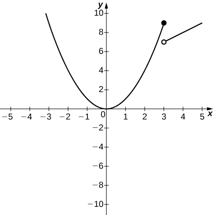 a. 9; b. 7
11. [T] [latex]g(x)=\begin{cases} x^3 - 1 & x \le 0 \\ 1 & x > 0 \end{cases}[/latex]
- [latex]\underset{x\to 0^-}{\lim}g(x)[/latex]
- [latex]\underset{x\to 0^+}{\lim}g(x)[/latex]
12. [T] [latex]h(x)=\begin{cases} x^2-2x+1 & x < 2 \\ 3 - x & x \ge 2 \end{cases}[/latex]
-
- [latex]\underset{x\to 2^-}{\lim}h(x)[/latex]
- [latex]\underset{x\to 2^+}{\lim}h(x)[/latex]
Answer: 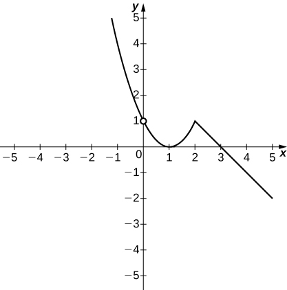 a. 1; b. 1
In the following exercises, use the following graphs and the limit laws to evaluate each limit.
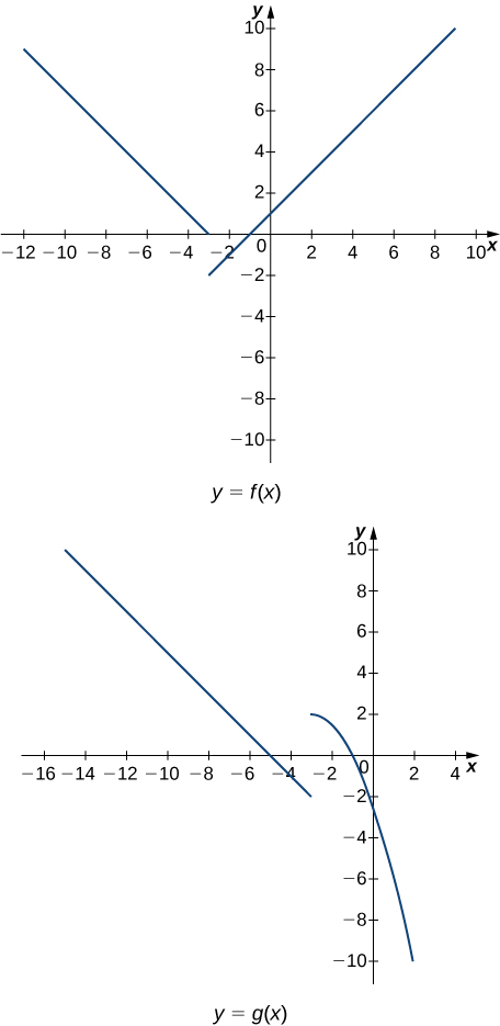
13. [latex]\underset{x\to -3^+}{\lim}(f(x)+g(x))[/latex]
14. [latex]\underset{x\to -3^-}{\lim}(f(x)-3g(x))[/latex]
Answer:
[latex]\underset{x\to -3^-}{\lim}(f(x)-3g(x))=\underset{x\to -3^-}{\lim}f(x)-3\underset{x\to -3^-}{\lim}g(x)=0+6=6[/latex]
In the following exercises, consider the graph of the function [latex]y=f(x)[/latex] shown here. Which of the statements about [latex]y=f(x)[/latex] are true and which are false? Explain why a statement is false.
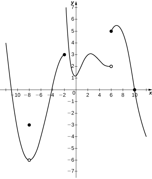
15. [latex]\underset{x\to 10^-}{\lim}f(x)=0[/latex]
16. [latex]\underset{x\to -2^+}{\lim}f(x)=3[/latex]
Answer:
False; [latex]\underset{x\to -2^+}{\lim}f(x)=+\infty [/latex]
17. [latex]\underset{x\to -8^+}{\lim}f(x)=f(-8)[/latex]
18. [latex]\underset{x\to 6}{\lim}f(x)=5[/latex]
Answer:
False; [latex]\underset{x\to 6}{\lim}f(x)[/latex] DNE since [latex]\underset{x\to 6^-}{\lim}f(x)=2[/latex] and [latex]\underset{x\to 6^+}{\lim}f(x)=5[/latex].
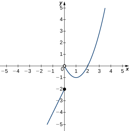
In the following exercises, use the following graph of the function [latex]y=f(x)[/latex] to find the values, if possible. Estimate when necessary.
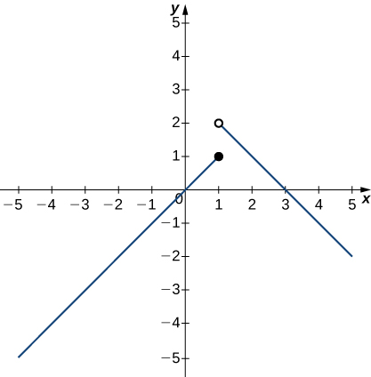
19. [latex]\underset{x\to 1^-}{\lim}f(x)[/latex]
Answer:
2
21. [latex]\underset{x\to 1}{\lim}f(x)[/latex]
In the following exercises, use the graph of the function [latex]y=f(x)[/latex] shown here to find the values, if possible. Estimate when necessary.
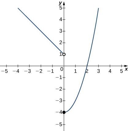
22. [latex]\underset{x\to 0^-}{\lim}f(x)[/latex]
Answer:
1
23. [latex]\underset{x\to 0^+}{\lim}f(x)[/latex]
24. [latex]\underset{x\to 2}{\lim}f(x)[/latex]
Answer:
DNE
25. [latex]\underset{x\to 2^-}{\lim}f(x)[/latex]
In the following exercises, use the graph of the function [latex]y=f(x)[/latex] shown here to find the values, if possible. Estimate when necessary.
![A graph of a piecewise function with three segments, all linear. The first exists for x < -2, has a slope of 1, and ends at the open circle at (-2, 0). The second exists over the interval [-2, 2], has a slope of -1, goes through the origin, and has closed circles at its endpoints (-2, 2) and (2,-2). The third exists for x>2, has a slope of 1, and begins at the open circle (2,2).](https://s3-us-west-2.amazonaws.com/courses-images/wp-content/uploads/sites/2332/2018/01/11202943/CNX_Calc_Figure_02_02_204.jpg)
26. [latex]\underset{x\to -2^-}{\lim}f(x)[/latex]
Answer:
0
27. [latex]\underset{x\to -2^+}{\lim}f(x)[/latex]
28. [latex]\underset{x\to -2}{\lim}f(x)[/latex]
Answer:
DNE
29. [latex]\underset{x\to 2^-}{\lim}f(x)[/latex]
30. [latex]\underset{x\to 2^+}{\lim}f(x)[/latex]
Answer:
2
31. [latex]\underset{x\to 2}{\lim}f(x)[/latex]
In the following exercises, use the graph of the function [latex]y=g(x)[/latex] shown here to find the values, if possible. Estimate when necessary.
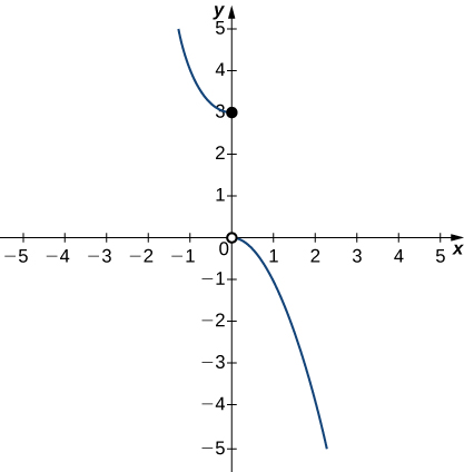
32. [latex]\underset{x\to 0^-}{\lim}g(x)[/latex]
Answer:
3
33. [latex]\underset{x\to 0^+}{\lim}g(x)[/latex]
34. [latex]\underset{x\to 0}{\lim}g(x)[/latex]
Answer:
DNE
In the following exercises, use the graph of the function [latex]y=h(x)[/latex] shown here to find the values, if possible. Estimate when necessary.
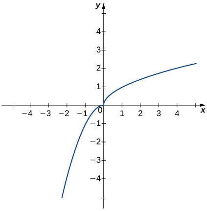
35. [latex]\underset{x\to 0^-}{\lim}h(x)[/latex]
36. [latex]\underset{x\to 0^+}{\lim}h(x)[/latex]
Answer:
0
37. [latex]\underset{x\to 0}{\lim}h(x)[/latex]
In the following exercises, use the graph of the function [latex]y=f(x)[/latex] shown here to find the values, if possible. Estimate when necessary.
38. [latex]\underset{x\to 0^-}{\lim}f(x)[/latex]
Answer:
−2
39. [latex]\underset{x\to 0^+}{\lim}f(x)[/latex]
40. [latex]\underset{x\to 0}{\lim}f(x)[/latex]
Answer:
DNE
41. [latex]\underset{x\to 1^-}{\lim}f(x)[/latex]
42. [latex]\underset{x\to 2^+}{\lim}f(x)[/latex]
Answer:
0
43. [latex]\underset{\theta \to 0}{\lim}\frac{\sin 2\theta}{5\theta}[/latex]
44. [latex]\underset{\theta \to 0}{\lim}\frac{\sin 4\theta}{3\theta}[/latex]
Answer:
[latex]\frac{4}{3}[/latex]
45. [latex]\underset{\theta \to 0}{\lim}\frac{1-\cos 2\theta}{9\theta}[/latex]
46. [latex]\underset{\theta \to 0}{\lim}\frac{1-\cos 2\theta}{3\theta}[/latex]
Answer:
[latex]0[/latex]
47. [latex]\underset{\theta \to 0}{\lim}\frac{\cos 2\theta+\sin 5\theta-1}{2\theta}[/latex]
48. [latex]\underset{\theta \to 0}{\lim}\frac{\cos 7\theta+\sin 2\theta-1}{7\theta}[/latex]
Answer:
[latex]\frac{2}{7}[/latex]
49. [latex]\underset{x \to 0}{\lim}\frac{x^2-x-\sin x}{3x}[/latex]
50. [latex]\underset{x \to 0}{\lim}\frac{x^2+x+\sin x}{4x}[/latex]
Answer:
[latex]\frac{1}{2}[/latex]
51. [latex]\underset{x \to 0}{\lim}\frac{\sin 5x}{\sin 4x}[/latex]
52. [latex]\underset{x \to 0}{\lim}\frac{\sin x}{\sin 2x}[/latex]
Answer:
[latex]\frac{1}{2}[/latex]

Hint