Linear Inequalities and Systems of Linear Inequalities in Two Variables
Learning Objectives
- Define solutions to a linear inequality in two variables
- Identify and follow steps for graphing a linear inequality in two variables
- Identify whether an ordered pair is in the solution set of a linear inequality
- Define solutions to systems of linear inequalities
- Graph a system of linear inequalities and define the solutions region
- Verify whether a point is a solution to a system of inequalities
- Identify when a system of inequalities has no solution
- Solutions from graphs of linear inequalities
- Solve systems of linear inequalities by graphing the solution region
- Graph solutions to a system that contains a compound inequality
- Applications of systems of linear inequalities
- Write and graph a system that models the quantity that must be sold to achieve a given amount of sales
- Write a system of inequalities that represents the profit region for a business
- Interpret the solutions to a system of cost/ revenue inequalities
Inequalities in two variables
Did you know that you use linear inequalities when you shop online? When you use the option to view items within a specific price range, you are asking the search engine to use a linear inequality based on price. Essentially, you are saying "show me all the items for sale between $50 and $100," which can be written as [latex]{50}\le {x} \le {100}[/latex], where x is price. In this section, you will apply what you know about graphing linear equations to graphing linear inequalities. So how do you get from the algebraic form of an inequality, like [latex]y>3x+1[/latex], to a graph of that inequality? Plotting inequalities is fairly straightforward if you follow a couple steps.Graphing Inequalities
To graph an inequality:- Graph the related boundary line. Replace the <, >, ≤ or ≥ sign in the inequality with = to find the equation of the boundary line.
- Identify at least one ordered pair on either side of the boundary line and substitute those [latex](x,y)[/latex] values into the inequality. Shade the region that contains the ordered pairs that make the inequality a true statement.
- If points on the boundary line are solutions, then use a solid line for drawing the boundary line. This will happen for ≤ or ≥ inequalities.
- If points on the boundary line aren’t solutions, then use a dotted line for the boundary line. This will happen for < or > inequalities.
| x | y |
| 0 | 1 |
| 4 | 0 |
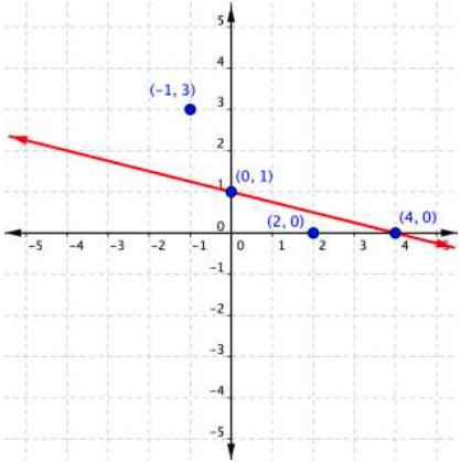 The next step is to find the region that contains the solutions. Is it above or below the boundary line? To identify the region where the inequality holds true, you can test a couple of ordered pairs, one on each side of the boundary line.
If you substitute [latex](−1,3)[/latex] into [latex]x+4y\leq4[/latex]:
The next step is to find the region that contains the solutions. Is it above or below the boundary line? To identify the region where the inequality holds true, you can test a couple of ordered pairs, one on each side of the boundary line.
If you substitute [latex](−1,3)[/latex] into [latex]x+4y\leq4[/latex]:
[latex]\begin{array}{r}−1+4\left(3\right)\leq4\\−1+12\leq4\\11\leq4\end{array}[/latex]
This is a false statement, since 11 is not less than or equal to 4. On the other hand, if you substitute [latex](2,0)[/latex] into [latex]x+4y\leq4[/latex]:[latex]\begin{array}{r}2+4\left(0\right)\leq4\\2+0\leq4\\2\leq4\end{array}[/latex]
This is true! The region that includes [latex](2,0)[/latex] should be shaded, as this is the region of solutions.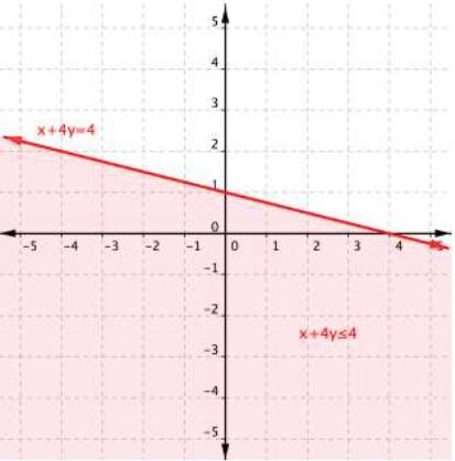 And there you have it—the graph of the set of solutions for [latex]x+4y\leq4[/latex].
Graphing Linear Inequalities in Two Variables
https://youtu.be/2VgFg2ztspIExample
Graph the inequality [latex]2y>4x–6[/latex].Answer: Solve for y.
[latex] \displaystyle \begin{array}{r}2y>4x-6\\\\\frac{2y}{2}>\frac{4x}{2}-\frac{6}{2}\\\\y>2x-3\\\end{array}[/latex]
Create a table of values to find two points on the line [latex] \displaystyle y=2x-3[/latex], or graph it based on the slope-intercept method, the b value of the y-intercept is [latex]-3[/latex] and the slope is 2. Plot the points, and graph the line. The line is dotted because the sign in the inequality is >, not ≥ and therefore points on the line are not solutions to the inequality.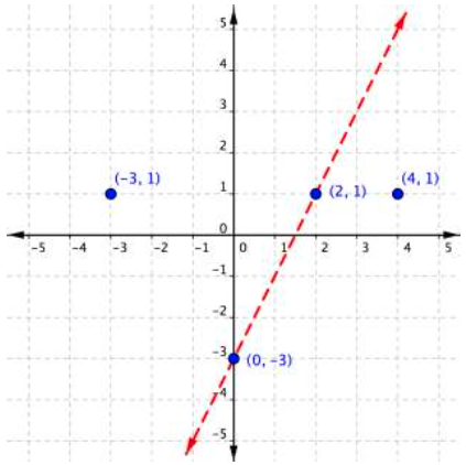
[latex] \displaystyle y=2x-3[/latex]
| x | y |
|---|---|
| 0 | [latex]−3[/latex] |
| 2 | 1 |
[latex]\begin{array}{l}2y>4x–6\\\\\text{Test }1:\left(−3,1\right)\\2\left(1\right)>4\left(−3\right)–6\\\,\,\,\,\,\,\,2>–12–6\\\,\,\,\,\,\,\,2>−18\\\text{TRUE}\\\\\text{Test }2:\left(4,1\right)\\2(1)>4\left(4\right)– 6\\\,\,\,\,\,\,2>16–6\\\,\,\,\,\,\,2>10\\\text{FALSE}\end{array}[/latex]
Answer
The graph of the inequality [latex]2y>4x–6[/latex] is: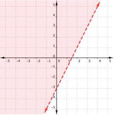
Solution Sets of Inequalities
The graph below shows the region of values that makes the inequality [latex]3x+2y\leq6[/latex] true (shaded red), the boundary line [latex]3x+2y=6[/latex], as well as a handful of ordered pairs. The boundary line is solid because points on the boundary line [latex]3x+2y=6[/latex] will make the inequality [latex]3x+2y\leq6[/latex] true.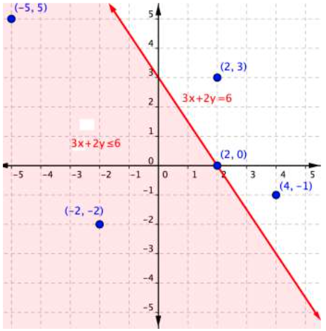 You can substitute the x- and y-values in each of the [latex](x,y)[/latex] ordered pairs into the inequality to find solutions. Sometimes making a table of values makes sense for more complicated inequalities.
| Ordered Pair | Makes the inequality [latex-display]3x+2y\leq6[/latex-display] a true statement | Makes the inequality [latex-display]3x+2y\leq6[/latex-display] a false statement |
|---|---|---|
| [latex](−5, 5)[/latex] | [latex]\begin{array}{r}3\left(−5\right)+2\left(5\right)\leq6\\−15+10\leq6\\−5\leq6\end{array}[/latex] | |
| [latex](−2,−2)[/latex] | [latex]\begin{array}{r}3\left(−2\right)+2\left(–2\right)\leq6\\−6+\left(−4\right)\leq6\\–10\leq6\end{array}[/latex] | |
| [latex](2,3)[/latex] | [latex]\begin{array}{r}3\left(2\right)+2\left(3\right)\leq6\\6+6\leq6\\12\leq6\end{array}[/latex] | |
| [latex](2,0)[/latex] | [latex]\begin{array}{r}3\left(2\right)+2\left(0\right)\leq6\\6+0\leq6\\6\leq6\end{array}[/latex] | |
| [latex](4,−1)[/latex] | [latex]\begin{array}{r}3\left(4\right)+2\left(−1\right)\leq6\\12+\left(−2\right)\leq6\\10\leq6\end{array}[/latex] |
Example
Use the graph to determine which ordered pairs plotted below are solutions of the inequality [latex]x–y<3[/latex].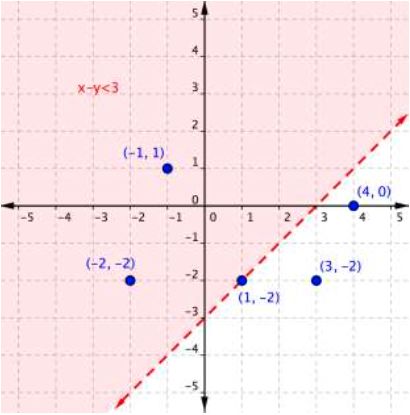
Answer: Solutions will be located in the shaded region. Since this is a “less than” problem, ordered pairs on the boundary line are not included in the solution set. These values are located in the shaded region, so are solutions. (When substituted into the inequality [latex]x–y<3[/latex], they produce true statements.)
[latex](−1,1)[/latex]
[latex](−2,−2)[/latex]
These values are not located in the shaded region, so are not solutions. (When substituted into the inequality [latex]x-y<3[/latex], they produce false statements.)[latex](1,−2)[/latex]
[latex](3,−2)[/latex]
[latex](4,0)[/latex]
Answer
[latex](−1,1)\,\,\,(−2,−2)[/latex]Example
Is [latex](2,−3)[/latex] a solution of the inequality [latex]y<−3x+1[/latex]?Answer: If [latex](2,−3)[/latex] is a solution, then it will yield a true statement when substituted into the inequality [latex]y<−3x+1[/latex].
[latex]y<−3x+1[/latex]
Substitute [latex]x=2[/latex] and [latex]y=−3[/latex] into inequality.[latex]−3<−3\left(2\right)+1[/latex]
Evaluate.[latex]\begin{array}{l}−3<−6+1\\−3<−5\end{array}[/latex]
This statement is not true, so the ordered pair [latex](2,−3)[/latex] is not a solution.Answer
[latex](2,−3)[/latex] is not a solution.Graph a system of two inequalities
Consider the graph of the inequality [latex]y<2x+5[/latex]. The dashed line is [latex]y=2x+5[/latex]. Every ordered pair in the shaded area below the line is a solution to [latex]y<2x+5[/latex], as all of the points below the line will make the inequality true. If you doubt that, try substituting the x and y coordinates of Points A and B into the inequality—you’ll see that they work. So, the shaded area shows all of the solutions for this inequality.
The boundary line divides the coordinate plane in half. In this case, it is shown as a dashed line as the points on the line don’t satisfy the inequality. If the inequality had been [latex]y\leq2x+5[/latex], then the boundary line would have been solid.
Let’s graph another inequality: [latex]y>−x[/latex]. You can check a couple of points to determine which side of the boundary line to shade. Checking points M and N yield true statements. So, we shade the area above the line. The line is dashed as points on the line are not true.
The dashed line is [latex]y=2x+5[/latex]. Every ordered pair in the shaded area below the line is a solution to [latex]y<2x+5[/latex], as all of the points below the line will make the inequality true. If you doubt that, try substituting the x and y coordinates of Points A and B into the inequality—you’ll see that they work. So, the shaded area shows all of the solutions for this inequality.
The boundary line divides the coordinate plane in half. In this case, it is shown as a dashed line as the points on the line don’t satisfy the inequality. If the inequality had been [latex]y\leq2x+5[/latex], then the boundary line would have been solid.
Let’s graph another inequality: [latex]y>−x[/latex]. You can check a couple of points to determine which side of the boundary line to shade. Checking points M and N yield true statements. So, we shade the area above the line. The line is dashed as points on the line are not true.
 To create a system of inequalities, you need to graph two or more inequalities together. Let’s use [latex]y<2x+5[/latex] and [latex]y>−x[/latex] since we have already graphed each of them.
 The purple area shows where the solutions of the two inequalities overlap. This area is the solution to the system of inequalities. Any point within this purple region will be true for both [latex]y>−x[/latex] and [latex]y<2x+5[/latex].
In the following video examples, we show how to graph a system of linear inequalities, and define the solution region.
https://youtu.be/ACTxJv1h2_c
https://youtu.be/cclH2h1NurM
In the next section, we will see that points can be solutions to systems of equations and inequalities. We will verify algebraically whether a point is a solution to a linear equation or inequality.
The purple area shows where the solutions of the two inequalities overlap. This area is the solution to the system of inequalities. Any point within this purple region will be true for both [latex]y>−x[/latex] and [latex]y<2x+5[/latex].
In the following video examples, we show how to graph a system of linear inequalities, and define the solution region.
https://youtu.be/ACTxJv1h2_c
https://youtu.be/cclH2h1NurM
In the next section, we will see that points can be solutions to systems of equations and inequalities. We will verify algebraically whether a point is a solution to a linear equation or inequality.
Determine whether an ordered pair is a solution to a system of linear inequalities
 On the graph above, you can see that the points B and N are solutions for the system because their coordinates will make both inequalities true statements.
In contrast, points M and A both lie outside the solution region (purple). While point M is a solution for the inequality [latex]y>−x[/latex] and point A is a solution for the inequality [latex]y<2x+5[/latex], neither point is a solution for the system. The following example shows how to test a point to see whether it is a solution to a system of inequalities.
On the graph above, you can see that the points B and N are solutions for the system because their coordinates will make both inequalities true statements.
In contrast, points M and A both lie outside the solution region (purple). While point M is a solution for the inequality [latex]y>−x[/latex] and point A is a solution for the inequality [latex]y<2x+5[/latex], neither point is a solution for the system. The following example shows how to test a point to see whether it is a solution to a system of inequalities.
Example
Is the point (2, 1) a solution of the system [latex]x+y>1[/latex] and [latex]2x+y<8[/latex]?Answer: Check the point with each of the inequalities. Substitute 2 for x and 1 for y. Is the point a solution of both inequalities? [latex-display]\begin{array}{r}x+y>1\\2+1>1\\3>1\\\text{TRUE}\end{array}[/latex-display] (2, 1) is a solution for [latex]x+y>1[/latex]. [latex-display]\begin{array}{r}2x+y<8\\2\left(2\right)+1<8\\4+1<8\\5<8\\\text{TRUE}\end{array}[/latex-display] (2, 1) is a solution for [latex]2x+y<8.[/latex] Since (2, 1) is a solution of each inequality, it is also a solution of the system.
Answer
The point (2, 1) is a solution of the system [latex]x+y>1[/latex] and [latex]2x+y<8[/latex].
Example
Is the point (2, 1) a solution of the system [latex]x+y>1[/latex] and [latex]3x+y<4[/latex]?Answer: Check the point with each of the inequalities. Substitute 2 for x and 1 for y. Is the point a solution of both inequalities? [latex-display]\begin{array}{r}x+y>1\\2+1>1\\3>1\\\text{TRUE}\end{array}[/latex-display] (2, 1) is a solution for [latex]x+y>1[/latex]. [latex-display]\begin{array}{r}3x+y<4\\3\left(2\right)+1<4\\6+1<4\\7<4\\\text{FALSE}\end{array}[/latex-display] (2, 1) is not a solution for [latex]3x+y<4[/latex]. Since (2, 1) is not a solution of one of the inequalities, it is not a solution of the system.
Answer
The point (2, 1) is not a solution of the system [latex]x+y>1[/latex] and [latex]3x+y<4[/latex]. In the following video we show another example of determining whether a point is in the solution of a system of linear inequalities.
https://youtu.be/o9hTFJEBcXs
As shown above, finding the solutions of a system of inequalities can be done by graphing each inequality and identifying the region they share. Below, you are given more examples that show the entire process of defining the region of solutions on a graph for a system of two linear inequalities. The general steps are outlined below:
In the following video we show another example of determining whether a point is in the solution of a system of linear inequalities.
https://youtu.be/o9hTFJEBcXs
As shown above, finding the solutions of a system of inequalities can be done by graphing each inequality and identifying the region they share. Below, you are given more examples that show the entire process of defining the region of solutions on a graph for a system of two linear inequalities. The general steps are outlined below:
- Graph each inequality as a line and determine whether it will be solid or dashed
- Determine which side of each boundary line represents solutions to the inequality by testing a point on each side
- Shade the region that represents solutions for both inequalities
Systems with no solutions
In the next example, we will show the solution to a system of two inequalities whose boundary lines are parallel to each other. When the graphs of a system of two linear equations are parallel to each other, we found that there was no solution to the system. We will get a similar result for the following system of linear inequalities.Examples
Graph the system [latex]\begin{array}{c}y\ge2x+1\\y\lt2x-3\end{array}[/latex]Answer: The boundary lines for this system are parallel to each other, note how they have the same slopes.
[latex]\begin{array}{c}y=2x+1\\y=2x-3\end{array}[/latex]
Plotting the boundary lines will give the graph below. Note that the inequality [latex]y\lt2x-3[/latex] requires that we draw a dashed line, while the inequality [latex]y\ge2x+1[/latex] will require a solid line.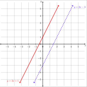 Now we need to add the regions that represent the inequalities. For the inequality [latex]y\ge2x+1[/latex] we can test a point on either side of the line to see which region to shade. Let's test [latex]\left(0,0\right)[/latex] to make it easy.
Substitute [latex]\left(0,0\right)[/latex] into [latex]y\ge2x+1[/latex]
Now we need to add the regions that represent the inequalities. For the inequality [latex]y\ge2x+1[/latex] we can test a point on either side of the line to see which region to shade. Let's test [latex]\left(0,0\right)[/latex] to make it easy.
Substitute [latex]\left(0,0\right)[/latex] into [latex]y\ge2x+1[/latex]
[latex]\begin{array}{c}y\ge2x+1\\0\ge2\left(0\right)+1\\0\ge{1}\end{array}[/latex]
This is not true, so we know that we need to shade the other side of the boundary line for the inequality [latex]y\ge2x+1[/latex]. The graph will now look like this: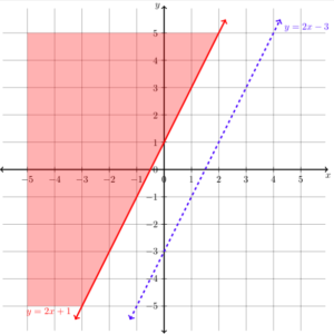 Now let's shade the region that shows the solutions to the inequality [latex]y\lt2x-3[/latex]. Again, we can pick [latex]\left(0,0\right)[/latex] to test because it makes easy algebra.
Substitute [latex]\left(0,0\right)[/latex] into [latex]y\lt2x-3[/latex]
Now let's shade the region that shows the solutions to the inequality [latex]y\lt2x-3[/latex]. Again, we can pick [latex]\left(0,0\right)[/latex] to test because it makes easy algebra.
Substitute [latex]\left(0,0\right)[/latex] into [latex]y\lt2x-3[/latex]
[latex]\begin{array}{c}y\lt2x-3\\0\lt2\left(0,\right)x-3\\0\lt{-3}\end{array}[/latex]
This is not true, so we know that we need to shade the other side of the boundary line for the inequality[latex]y\lt2x-3[/latex]. The graph will now look like this: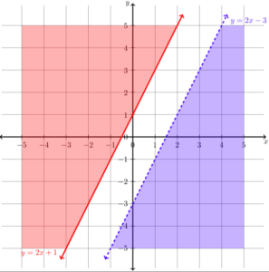 This system of inequalities shares no points in common.
Example
Shade the region of the graph that represents solutions for both inequalities. [latex]x+y\geq1[/latex] and [latex]y–x\geq5[/latex].Answer: Graph one inequality. First graph the boundary line, using a table of values, intercepts, or any other method you prefer. The boundary line for [latex]x+y\geq1[/latex] is [latex]x+y=1[/latex], or [latex]y=−x+1[/latex]. Since the equal sign is included with the greater than sign, the boundary line is solid.
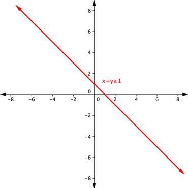 Find an ordered pair on either side of the boundary line. Insert the x- and y-values into the inequality [latex]x+y\geq1[/latex] and see which ordered pair results in a true statement.
[latex-display]\begin{array}{r}\text{Test }1:\left(−3,0\right)\\x+y\geq1\\−3+0\geq1\\−3\geq1\\\text{FALSE}\\\\\text{Test }2:\left(4,1\right)\\x+y\geq1\\4+1\geq1\\5\geq1\\\text{TRUE}\end{array}[/latex-display]
Since (4, 1) results in a true statement, the region that includes (4, 1) should be shaded.
Find an ordered pair on either side of the boundary line. Insert the x- and y-values into the inequality [latex]x+y\geq1[/latex] and see which ordered pair results in a true statement.
[latex-display]\begin{array}{r}\text{Test }1:\left(−3,0\right)\\x+y\geq1\\−3+0\geq1\\−3\geq1\\\text{FALSE}\\\\\text{Test }2:\left(4,1\right)\\x+y\geq1\\4+1\geq1\\5\geq1\\\text{TRUE}\end{array}[/latex-display]
Since (4, 1) results in a true statement, the region that includes (4, 1) should be shaded.
 Do the same with the second inequality. Graph the boundary line, then test points to find which region is the solution to the inequality. In this case, the boundary line is [latex]y–x=5\left(\text{or }y=x+5\right)[/latex] and is solid. Test point (−3, 0) is not a solution of [latex]y–x\geq5[/latex], and test point (0, 6) is a solution.

Answer
The purple region in this graph shows the set of all solutions of the system.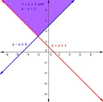
Example
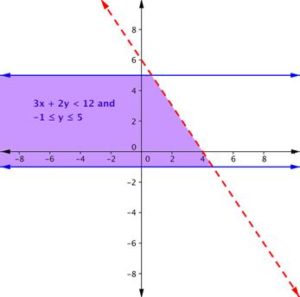
Find the solution to the system 3x + 2y < 12 and −1 ≤ y ≤ 5.Answer:
Graph one inequality. First graph the boundary line, then test points.
Remember, because the inequality 3x + 2y < 12 does not include the equal sign, draw a dashed border line.
Testing a point (like (0, 0) will show that the area below the line is the solution to this inequality.
 The inequality −1 ≤ y ≤ 5 is actually two inequalities: −1 ≤ y, and y ≤ 5. Another way to think of this is y must be between −1 and 5. The border lines for both are horizontal. The region between those two lines contains the solutions of −1 ≤ y ≤ 5. We make the lines solid because we also want to include y = −1 and y = 5.
Graph this region on the same axes as the other inequality.
The inequality −1 ≤ y ≤ 5 is actually two inequalities: −1 ≤ y, and y ≤ 5. Another way to think of this is y must be between −1 and 5. The border lines for both are horizontal. The region between those two lines contains the solutions of −1 ≤ y ≤ 5. We make the lines solid because we also want to include y = −1 and y = 5.
Graph this region on the same axes as the other inequality.
 The purple region in this graph shows the set of all solutions of the system.
Answer
Applications
In our first example we will show how to write and graph a system of linear inequalities that models the amount of sales needed to obtain a specific amount of money.Example
Cathy is selling ice cream cones at a school fundraiser. She is selling two sizes: small (which has 1 scoop) and large (which has 2 scoops). She knows that she can get a maximum of 70 scoops of ice cream out of her supply. She charges $3 for a small cone and $5 for a large cone. Cathy wants to earn at least $120 to give back to the school. Write and graph a system of inequalities that models this situation.Answer: First, identify the variables. There are two variables: the number of small cones and the number of large cones.
s = small cone
l = large cone
Write the first equation: the maximum number of scoops she can give out. The scoops she has available (70) must be greater than or equal to the number of scoops for the small cones (s) and the large cones (2l) she sells.
[latex]s+2l\le70[/latex]
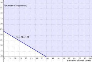
Write the second equation: the amount of money she raises. She wants the total amount of money earned from small cones (3s) and large cones (5l) to be at least $120.
[latex]3s+5l\ge120[/latex]
Write the system.
[latex]\begin{cases}s+2l\le70\\3s+5l\ge120\end{cases}[/latex]
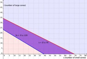
Now graph the system. The variables x and y have been replaced by s and l; graph s along the x-axis, and l along the y-axis. First graph the region s + 2l ≤ 70. Graph the boundary line and then test individual points to see which region to shade. The graph is shown below.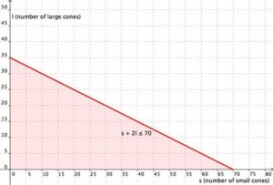 Now graph the region [latex]3s+5l\ge120[/latex] Graph the boundary line and then test individual points to see which region to shade. The graph is shown below.
 Graphing the regions together, you find the following:
 And represented just as the overlapping region, you have:
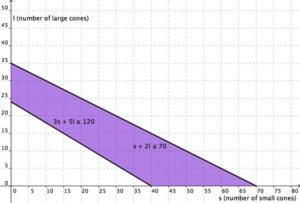
Answer
The region in purple is the solution. As long as the combination of small cones and large cones that Cathy sells can be mapped in the purple region, she will have earned at least $120 and not used more than 70 scoops of ice cream.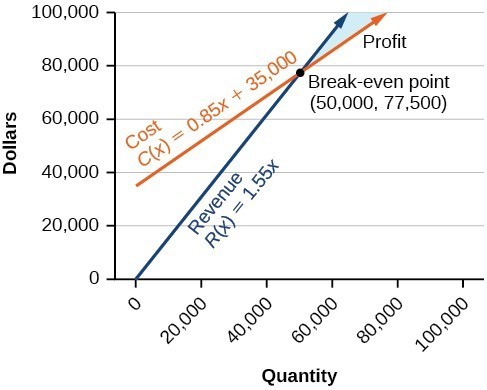 Note how the blue shaded region between the Cost and Revenue equations is labeled Profit. This is the "sweet spot" that the company wants to achieve where they produce enough bike frames at a minimal enough cost to make money. They don't want more money going out than coming in!
Example
Define the profit region for the skateboard manufacturing business using inequalities, given the system of linear equations: Cost: [latex]y=0.85x+35,000[/latex] Revenue: [latex]y=1.55x[/latex]Answer:
We know that graphically, solutions to linear inequalities are entire regions, and we learned how to graph systems of linear inequalities earlier in this module. Based on the graph below and the equations that define cost and revenue, we can use inequalities to define the region for which the skateboard manufacturer will make a profit.
 Let's start with the revenue equation. We know that the break even point is at (50,000, 77,500) and the profit region is the blue area. If we choose a point in the region and test it like we did for finding solution regions to inequalities, we will know which kind of inequality sign to use.
Let's test the point [latex]\left(65,00,100,000\right)[/latex] in both equations to determine which inequality sign to use.
Cost:
Let's start with the revenue equation. We know that the break even point is at (50,000, 77,500) and the profit region is the blue area. If we choose a point in the region and test it like we did for finding solution regions to inequalities, we will know which kind of inequality sign to use.
Let's test the point [latex]\left(65,00,100,000\right)[/latex] in both equations to determine which inequality sign to use.
Cost:
[latex]\begin{array}{l}y=0.85x+{35,000}\\{100,000}\text{ ? }0.85\left(65,000\right)+35,000\\100,000\text{ ? }90,250\end{array}[/latex]
We need to use > because 100,000 is greater than 90,250 The cost inequality that will ensure the company makes profit - not just break even - is [latex]y>0.85x+35,000[/latex] Now test the point in the revenue equation: Revenue:[latex]\begin{array}{l}y=1.55x\\100,000\text{ ? }1.55\left(65,000\right)\\100,000\text{ ? }100,750\end{array}[/latex]
We need to use < because 100,000 is less than 100,750 The revenue inequality that will ensure the company makes profit - not just break even - is [latex]y<1.55x[/latex] The systems of inequalities that defines the profit region for the bike manufacturer:[latex]\begin{array}{l}y>0.85x+35,000\\y<1.55x\end{array}[/latex]
Answer
The cost to produce 50,000 units is $77,500, and the revenue from the sales of 50,000 units is also $77,500. To make a profit, the business must produce and sell more than 50,000 units. The system of linear inequalities that represents the number of units that the company must produce in order to earn a profit is: [latex-display]\begin{array}{l}y>0.85x+35,000\\y<1.55x\end{array}[/latex-display]Licenses & Attributions
CC licensed content, Original
- Ex 1: Graphing Linear Inequalities in Two Variables (Slope Intercept Form). Authored by: James Sousa (Mathispower4u.com) . License: CC BY: Attribution.
- System of Equations App: Break-Even Point.. Authored by: James Sousa (Mathispower4u.com) for Lumen Learning. License: CC BY: Attribution.
- Revision and Adaptation. Provided by: Lumen Learning License: CC BY: Attribution.
CC licensed content, Shared previously
- Ex 2: Graphing Linear Inequalities in Two Variables (Standard Form). Authored by: James Sousa (Mathispower4u.com) . License: CC BY: Attribution.
- Unit 13: Graphing, from Developmental Math: An Open Program. Provided by: Monterey Institute of Technology and Education Located at: https://www.nroc.org/. License: CC BY: Attribution.
- Use a Graph Determine Ordered Pair Solutions of a Linear Inequalty in Two Variable. Authored by: James Sousa (Mathispower4u.com) for Lumen Learning. License: CC BY: Attribution.
- Ex: Determine if Ordered Pairs Satisfy a Linear Inequality. Authored by: James Sousa (Mathispower4u.com) . License: CC BY: Attribution.
- Ex 1: Graph a System of Linear Inequalities. . Authored by: James Sousa (Mathispower4u.com) .. License: CC BY: Attribution.
- Ex 2: Graph a System of Linear Inequalities.. Authored by: James Sousa (Mathispower4u.com). License: CC BY: Attribution.
- Unit 14: Systems of Equations and Inequalities, from Developmental Math: An Open Program.. Provided by: Monterey Institute of Technology. Located at: https://www.nroc.org/. License: CC BY: Attribution.
- Determine the Solution to a System of Inequalities (Compound).. Authored by: James Sousa (Mathispower4u.com) . License: CC BY: Attribution.
- College Algebra. Provided by: OpenStax Authored by: Jay Abrams, et al.. Located at: https://openstax.org/textbooks/college-algebra.. License: CC BY: Attribution.
