Local Behavior of Polynomial Functions
Learning Outcomes
- Identify turning points of a polynomial function from its graph.
- Identify the number of turning points and intercepts of a polynomial function from its degree.
- Determine x and y-intercepts of a polynomial function given its equation in factored form.
Identifying Local Behavior of Polynomial Functions
In addition to the end behavior of polynomial functions, we are also interested in what happens in the "middle" of the function. In particular, we are interested in locations where graph behavior changes. A turning point is a point at which the function values change from increasing to decreasing or decreasing to increasing.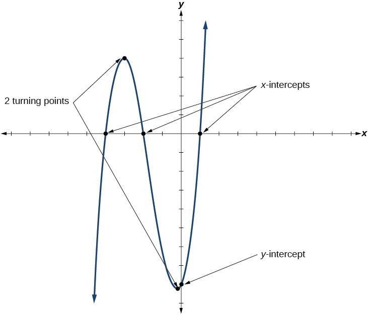 We are also interested in the intercepts. As with all functions, the y-intercept is the point at which the graph intersects the vertical axis. The point corresponds to the coordinate pair in which the input value is zero. Because a polynomial is a function, only one output value corresponds to each input value so there can be only one y-intercept [latex]\left(0,{a}_{0}\right)[/latex]. The x-intercepts occur at the input values that correspond to an output value of zero. It is possible to have more than one x-intercept.
A General Note: Intercepts and Turning Points of Polynomial Functions
- A turning point of a graph is a point where the graph changes from increasing to decreasing or decreasing to increasing.
- The y-intercept is the point where the function has an input value of zero.
- The x-intercepts are the points where the output value is zero.
- A polynomial of degree n will have, at most, n x-intercepts and n – 1 turning points.
Determining the Number of Turning Points and Intercepts from the Degree of the Polynomial
A continuous function has no breaks in its graph: the graph can be drawn without lifting the pen from the paper. A smooth curve is a graph that has no sharp corners. The turning points of a smooth graph must always occur at rounded curves. The graphs of polynomial functions are both continuous and smooth. The degree of a polynomial function helps us to determine the number of x-intercepts and the number of turning points. A polynomial function of nth degree is the product of n factors, so it will have at most n roots or zeros, or x-intercepts. The graph of the polynomial function of degree n must have at most n – 1 turning points. This means the graph has at most one fewer turning point than the degree of the polynomial or one fewer than the number of factors.tip for success
Why do we use the phrase "at most [latex]n[/latex]" when describing the number of real roots (x-intercepts) of the graph of an [latex]n^{\text{th}}[/latex] degree polynomial? Can it have fewer?Answer: Ex. Consider the graph of the polynomial function [latex]f(x)=x^2-x+1[/latex]. The function is a [latex]2^{\text{nd}}[/latex] degree polynomial, so it must have at most [latex]n[/latex] roots and [latex]n-1[/latex] turning points. We know this function has non-real roots since the discriminant of the quadratic formula is negative. This means that this [latex]2^{\text{nd}}[/latex] polynomial has no real roots (apply the quadratic formula to prove this to yourself if needed). That is, it has no x-intercepts. But it does have two distinct complex roots. Can you picture the graph of a quadratic function with one distinct real root? Two? But you can also see that there will never be more than two x-intercepts. Since a parabola (the graph of a [latex]2^{\text{nd}}[/latex] degree polynomial) has only one turning point, it can't cross the x-axis more than twice.
Example: Determining the Number of Intercepts and Turning Points of a Polynomial
Without graphing the function, determine the local behavior of the function by finding the maximum number of x-intercepts and turning points for [latex]f\left(x\right)=-3{x}^{10}+4{x}^{7}-{x}^{4}+2{x}^{3}[/latex].Answer: The polynomial has a degree of 10, so there are at most 10 x-intercepts and at most [latex]10 – 1 = 9[/latex] turning points.
Try It
Without graphing the function, determine the maximum number of x-intercepts and turning points for [latex]f\left(x\right)=108 - 13{x}^{9}-8{x}^{4}+14{x}^{12}+2{x}^{3}[/latex]Answer: There are at most 12 x-intercepts and at most 11 turning points.
[ohm_question]123739[/ohm_question]How To: Given a polynomial function, determine the intercepts
- Determine the y-intercept by setting [latex]x=0[/latex] and finding the corresponding output value.
- Determine the x-intercepts by setting the function equal to zero and solving for the input values.
Using the Principle of Zero Products to Find the Roots of a Polynomial in Factored Form
The Principle of Zero Products states that if the product of n numbers is 0, then at least one of the factors is 0. If [latex]ab=0[/latex], then either [latex]a=0[/latex] or [latex]b=0[/latex], or both a and b are 0. We will use this idea to find the zeros of a polynomial that is either in factored form or can be written in factored form. For example, the polynomial[latex]P(x)=(x-4)^2(x+1)(x-7)[/latex]
is in factored form. In the following examples, we will show the process of factoring a polynomial and calculating its x and y-intercepts.Example: Determining the Intercepts of a Polynomial Function
Given the polynomial function [latex]f\left(x\right)=\left(x - 2\right)\left(x+1\right)\left(x - 4\right)[/latex], written in factored form for your convenience, determine the y and x-intercepts.Answer: The y-intercept occurs when the input is zero, so substitute 0 for x.
[latex]\begin{array}{l}f\left(0\right)=\left(0 - 2\right)\left(0+1\right)\left(0 - 4\right)\hfill \\ \text{}f\left(0\right)=\left(-2\right)\left(1\right)\left(-4\right)\hfill \\ \text{}f\left(0\right)=8\hfill \end{array}[/latex]
The y-intercept is (0, 8). The x-intercepts occur when the output [latex]f(x)[/latex] is zero.[latex]0=\left(x - 2\right)\left(x+1\right)\left(x - 4\right)[/latex]
[latex]\begin{array}{llllllllllll}x - 2=0\hfill & \hfill & \text{or}\hfill & \hfill & x+1=0\hfill & \hfill & \text{or}\hfill & \hfill & x - 4=0\hfill \\ \text{}x=2\hfill & \hfill & \text{or}\hfill & \hfill & \text{ }x=-1\hfill & \hfill & \text{or}\hfill & \hfill & x=4 \end{array}[/latex]
The x-intercepts are [latex]\left(2,0\right),\left(-1,0\right)[/latex], and [latex]\left(4,0\right)[/latex]. We can see these intercepts on the graph of the function shown below.
Example: Determining the Intercepts of a Polynomial Function BY Factoring
Given the polynomial function [latex]f\left(x\right)={x}^{4}-4{x}^{2}-45[/latex], determine the y and x-intercepts.Answer: The y-intercept occurs when the input is zero.
[latex]\begin{array}{l} \\ f\left(0\right)={\left(0\right)}^{4}-4{\left(0\right)}^{2}-45\hfill \hfill \\ \text{}f\left(0\right)=-45\hfill \end{array}[/latex]
The y-intercept is [latex]\left(0,-45\right)[/latex]. The x-intercepts occur when the output is zero. To determine when the output is zero, we will need to factor the polynomial.[latex]\begin{array}{l}f\left(x\right)={x}^{4}-4{x}^{2}-45\hfill \\ f\left(x\right)=\left({x}^{2}-9\right)\left({x}^{2}+5\right)\hfill \\ f\left(x\right)=\left(x - 3\right)\left(x+3\right)\left({x}^{2}+5\right)\hfill \end{array}[/latex]
Then set the polynomial function equal to 0.[latex]0=\left(x - 3\right)\left(x+3\right)\left({x}^{2}+5\right)[/latex]
[latex]\begin{array}{lllllllll}x - 3=0\hfill & \text{or}\hfill & x+3=0\hfill & \text{or}\hfill & {x}^{2}+5=0\hfill \\ \text{}x=3\hfill & \text{or}\hfill & \text{}x=-3\hfill & \text{or}\hfill & \text{(no real solution)}\hfill \end{array}[/latex]
The x-intercepts are [latex]\left(3,0\right)[/latex] and [latex]\left(-3,0\right)[/latex]. We can see these intercepts on the graph of the function shown below. We can see that the function has y-axis symmetry or is even because [latex]f\left(x\right)=f\left(-x\right)[/latex].
recall special factoring techniques
In the example above, you needed to factor a [latex]4^{\text{th}}[/latex] polynomial in order to use the zero-product principle. Some, but not all, polynomials of degree higher than [latex]2[/latex] are factorable using special techniques you learned earlier in the course. What technique was used to factor [latex]x^4-4x^2-45[/latex]?Answer: First, we can recognize that the smallest power in this trinomial is exactly half the larger power. This allows us to make a substitution. We can let [latex]u=x^2[/latex]. Then [latex]u^2 = x^4[/latex]. We now have the factorable quadratic equation [latex]\begin{align} 0 &= u^2-4u-45 \\ 0 &= (u-9)(u+5)\end{align}[/latex]. Back substituting [latex]u=x^2[/latex] into the function yields the factored form of the equation to which we can apply the zero-product principle. [latex]\begin{align}0 &= (x^2 - 9)(x^2+5) \\ 0 &= (x+3)(x-3)(x^2+5)\end{align}[/latex]. So, [latex]x=-3, 3, \text{ and } \pm \sqrt{5}i[/latex].
Try It
Given the polynomial function [latex]f\left(x\right)=2{x}^{3}-6{x}^{2}-20x[/latex], determine the y and x-intercepts.Answer: y-intercept [latex]\left(0,0\right)[/latex]; x-intercepts [latex]\left(0,0\right),\left(-2,0\right)[/latex], and [latex]\left(5,0\right)[/latex]
The Whole Picture
Now we can bring the two concepts of turning points and intercepts together to get a general picture of the behavior of polynomial functions. These types of analyses on polynomials developed before the advent of mass computing as a way to quickly understand the general behavior of a polynomial function. We now have a quick way, with computers, to graph and calculate important characteristics of polynomials that once took a lot of algebra. In the first example, we will determine the least degree of a polynomial based on the number of turning points and intercepts.Example: Drawing Conclusions about a Polynomial Function from Its Graph
Given the graph of the polynomial function below, determine the least possible degree of the polynomial and whether it is even or odd. Use end behavior, the number of intercepts, and the number of turning points to help you.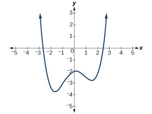
Answer:
 The end behavior of the graph tells us this is the graph of an even-degree polynomial.
The graph has 2 x-intercepts, suggesting a degree of 2 or greater, and 3 turning points, suggesting a degree of 4 or greater. Based on this, it would be reasonable to conclude that the degree is even and at least 4.
The end behavior of the graph tells us this is the graph of an even-degree polynomial.
The graph has 2 x-intercepts, suggesting a degree of 2 or greater, and 3 turning points, suggesting a degree of 4 or greater. Based on this, it would be reasonable to conclude that the degree is even and at least 4.
Try It
Given the graph of the polynomial function below, determine the least possible degree of the polynomial and whether it is even or odd. Use end behavior, the number of intercepts, and the number of turning points to help you.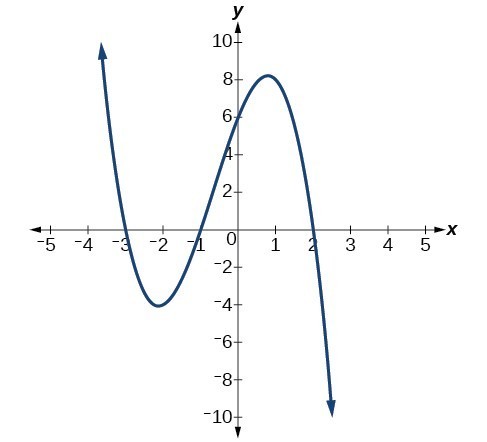
Answer: The end behavior indicates an odd-degree polynomial function; there are 3 x-intercepts and 2 turning points, so the degree is odd and at least 3. Because of the end behavior, we know that the leading coefficient must be negative.
[ohm_question]15937[/ohm_question]Example: Drawing Conclusions about a Polynomial Function from ITS Factors
Given the function [latex]f\left(x\right)=-4x\left(x+3\right)\left(x - 4\right)[/latex], determine the local behavior.Answer: The y-intercept is found by evaluating [latex]f\left(0\right)[/latex].
[latex]\begin{array}{c}f\left(0\right)=-4\left(0\right)\left(0+3\right)\left(0 - 4\right)\hfill \hfill \\ \text{}f\left(0\right)=0\hfill \end{array}[/latex]
The y-intercept is [latex]\left(0,0\right)[/latex]. The x-intercepts are found by setting the function equal to 0.[latex]0=-4x\left(x+3\right)\left(x - 4\right)[/latex]
[latex]\begin{array}{lllllllllllllll}-4x=0\hfill & \hfill & \text{or}\hfill & \hfill & x+3=0\hfill & \hfill & \text{or}\hfill & \hfill & x - 4=0\hfill \\ x=0\hfill & \hfill & \text{or}\hfill & \hfill & \text{}x=-3\hfill & \hfill & \text{or}\hfill & \hfill & \text{}x=4\end{array}[/latex]
The x-intercepts are [latex]\left(0,0\right),\left(-3,0\right)[/latex], and [latex]\left(4,0\right)[/latex]. The degree is 3 so the graph has at most 2 turning points.Try It
Given the function [latex]f\left(x\right)=0.2\left(x - 2\right)\left(x+1\right)\left(x - 5\right)[/latex], determine the local behavior.Answer: The x-intercepts are [latex]\left(2,0\right),\left(-1,0\right)[/latex], and [latex]\left(5,0\right)[/latex], the y-intercept is [latex]\left(0,\text{2}\right)[/latex], and the graph has at most 2 turning points.
Licenses & Attributions
CC licensed content, Original
- Revision and Adaptation. Provided by: Lumen Learning License: CC BY: Attribution.
- Question ID 123739. Provided by: Lumen Learning License: CC BY: Attribution. License terms: IMathAS Community License CC-BY + GPL.
CC licensed content, Shared previously
- Question ID 15937. Authored by: Sousa, James. License: Other. License terms: iMathAS/ WAMAP/ MyOpenMath Community License (GPL + CC-BY).
- Turning Points and X-Intercepts of a Polynomial Function. Authored by: Sousa, James (Mathispower4u). License: CC BY: Attribution.
- College Algebra. Provided by: OpenStax Authored by: Abramson, Jay et al.. Located at: https://openstax.org/books/college-algebra/pages/1-introduction-to-prerequisites. License: CC BY: Attribution. License terms: Download for free at http://cnx.org/contents/[email protected].
