Transformations
Transformations of Functions
Transformations alter a function while maintaining the original characteristics of that function.Learning Objectives
Determine whether a given transformation is an example of translation, scaling, rotation, or reflectionKey Takeaways
Key Points
- Transformations are ways that a function can be adjusted to create new functions.
- Transformations often preserve the original shape of the function.
- Common types of transformations include rotations, translations, reflections, and scaling (also known as stretching/shrinking).
Key Terms
- translation: Shift of an entire function in a specific direction.
- Scaling: Changes the size and/or the shape of the function.
- rotation: Spins the function around the origin.
- reflection: Mirror image of a function.
Translations
A translation moves every point by a fixed distance in the same direction. The movement is caused by the addition or subtraction of a constant from a function. As an example, let [latex]f(x) = x^3[/latex]. One possible translation of [latex]f(x)[/latex] would be [latex]x^3 + 2[/latex]. This would then be read as, "the translation of [latex]f(x)[/latex] by two in the positive y direction".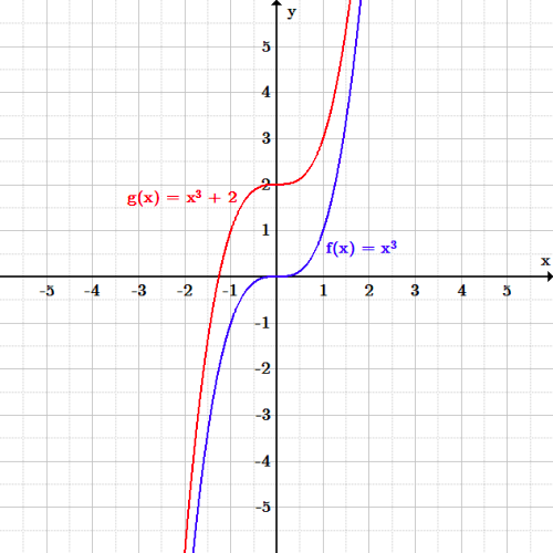 Graph of a function being translated: The function [latex]f(x)=x^3[/latex] is translated by two in the positive [latex]y[/latex] direction (up).
Reflections
A reflection of a function causes the graph to appear as a mirror image of the original function. This can be achieved by switching the sign of the input going into the function. Let the function in question be [latex]f(x) = x^5[/latex]. The mirror image of this function across the [latex]y[/latex]-axis would then be [latex]f(-x) = -x^5[/latex]. Therefore, we can say that [latex]f(-x)[/latex] is a reflection of [latex]f(x)[/latex] across the [latex]y[/latex]-axis.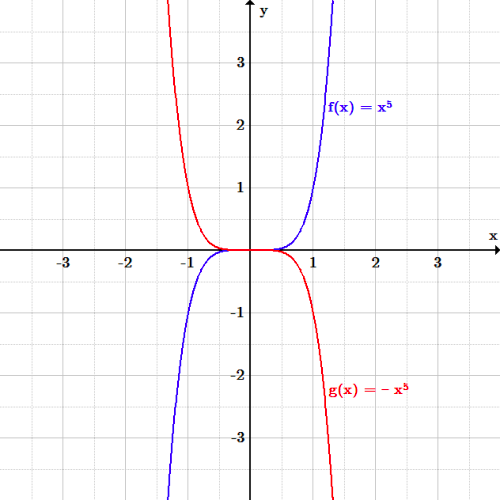 Graph of a function being reflected: The function [latex]f(x)=x^5[/latex] is reflected over the [latex]y[/latex]-axis.
Rotations
A rotation is a transformation that is performed by "spinning" the object around a fixed point known as the center of rotation. Although the concept is simple, it has the most advanced mathematical process of the transformations discussed. There are two formulas that are used: [latex-display]x_1 = x_0cos\theta - y_0sin\theta \\ y_1 = x_0sin\theta + y_0cos\theta[/latex-display] Where [latex]x_1[/latex]and [latex]y_1[/latex]are the new expressions for the rotated function, [latex]x_0[/latex] and [latex]y_0[/latex] are the original expressions from the function being transformed, and [latex]\theta[/latex] is the angle at which the function is to be rotated. As an example, let [latex]y=x^2[/latex]. If we rotate this function by 90 degrees, the new function reads: [latex-display][xsin(\frac{\pi}{2}) + ycos(\frac{\pi}{2})] = [xcos(\frac{\pi}{2}) - ysin(\frac{\pi}{2})]^2[/latex-display]Scaling
Scaling is a transformation that changes the size and/or the shape of the graph of the function. Note that until now, none of the transformations we discussed could change the size and shape of a function - they only moved the graphical output from one set of points to another set of points. As an example, let [latex]f(x) = x^3[/latex]. Following from this, [latex]2f(x) = 2x^3[/latex]. The graph has now physically gotten "taller", with every point on the graph of the original function being multiplied by two.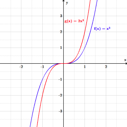 Graph of a function being scaled: The function [latex]f(x)=x^3[/latex] is scaled by a factor of two.
Translations
A translation of a function is a shift in one or more directions. It is represented by adding or subtracting from either y or x.Learning Objectives
Manipulate functions so that they are translated vertically and horizontallyKey Takeaways
Key Points
- A translation is a function that moves every point a constant distance in a specified direction.
- A vertical translation is generally given by the equation [latex]y=f(x)+b[/latex]. These translations shift the whole function up or down the y-axis.
- A horizontal translation is generally given by the equation [latex]y=f(x-a)[/latex]. These translations shift the whole function side to side on the x-axis.
Key Terms
- translation: A shift of the whole function by a specified amount.
- vertical translation: A shift of the function along the [latex]y[/latex]-axis.
- horizontal translation: A shift of the function along the [latex]x[/latex]-axis.
Vertical Translations
To translate a function vertically is to shift the function up or down. If a positive number is added, the function shifts up the [latex]y[/latex]-axis by the amount added. If a positive number is subtracted, the function shifts down the [latex]y[/latex]-axis by the amount subtracted. In general, a vertical translation is given by the equation: [latex]\displaystyle y = f(x) + b[/latex] where [latex]f(x)[/latex] is some given function and [latex]b[/latex] is the constant that we are adding to cause a translation. Let's use a basic quadratic function to explore vertical translations. The original function we will use is: [latex]\displaystyle y = x^2[/latex]. Translating the function up the [latex]y[/latex]-axis by two produces the equation: [latex]\displaystyle y=x^2 + 2[/latex] And translating the function down the [latex]y[/latex]-axis by two produces the equation: [latex]y=x^2 - 2[/latex].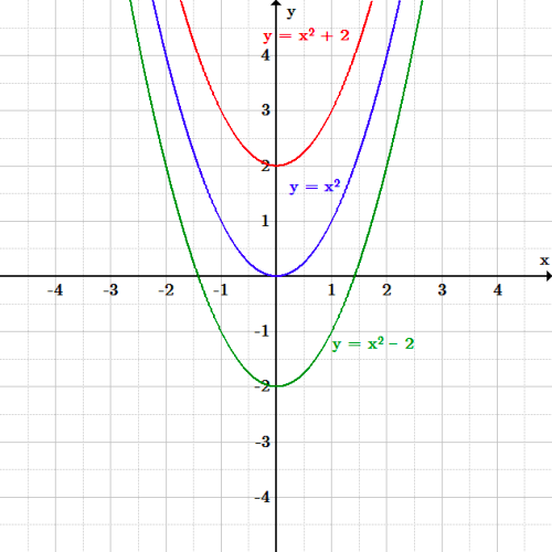 Vertical translations: The function [latex]f(x)=x^2[/latex] is translated both up and down by two.
Horizontal Translations
To translate a function horizontally is the shift the function left or right. While vertical shifts are caused by adding or subtracting a value outside of the function parameters, horizontal shifts are caused by adding or subtracting a value inside the function parameters. The general equation for a horizontal shift is given by: [latex]\displaystyle y = f(x-a)[/latex] Where [latex]f(x)[/latex] would be the original function, and [latex]a[/latex] is the constant being added or subtracted to cause a horizontal shift. When [latex]a[/latex] is positive, the function is shifted to the right. When [latex]a[/latex] is negative, the function is shifted to the left. Let's use the same basic quadratic function to look at horizontal translations. Again, the original function is: [latex]\displaystyle y = x^2[/latex]. Shifting the function to the left by two produces the equation: [latex]\displaystyle \begin{align} y &= f(x+2)\\ &= (x+2)^2 \end{align}[/latex] Shifting the function to the right by two produces the equation: [latex]\displaystyle \begin{align} y &= f(x-2)\\ & = (x-2)^2 \end{align}[/latex]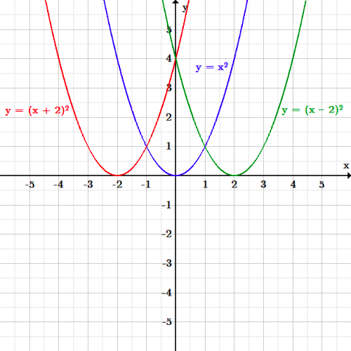 Horizontal translation: The function [latex]f(x)=x^2[/latex] is translated both left and right by two.
Reflections
Reflections are a type of transformation that move an entire curve such that its mirror image lies on the other side of the [latex]x[/latex] or [latex]y[/latex]-axis.Learning Objectives
Calculate the reflection of a function over the [latex]x[/latex]-axis, [latex]y[/latex]-axis, or the line [latex]y=x[/latex]Key Takeaways
Key Points
- A reflection swaps all of the [latex]x[/latex] or [latex]y[/latex] values across the [latex]x[/latex] or [latex]y[/latex]-axis, respectively. It can be visualized by imagining that a mirror lies across that axis.
- A vertical reflection is given by the equation [latex]y = -f(x)[/latex] and results in the curve being "reflected" across the x-axis.
- A horizontal reflection is given by the equation [latex]y = f(-x)[/latex] and results in the curve being "reflected" across the y-axis.
Key Terms
- Reflection: A mirror image of a function across a given line.
Vertical Reflections
A vertical reflection is a reflection across the [latex]x[/latex]-axis, given by the equation: [latex]\displaystyle y=-f(x)[/latex] In this general equation, all [latex]y[/latex] values are switched to their negative counterparts while the [latex]x[/latex] values remain the same. The result is that the curve becomes flipped over the [latex]x[/latex]-axis. As an example, let the original function be: [latex]\displaystyle y = x^2[/latex] The vertical reflection would then produce the equation: [latex]\displaystyle \begin{align} y &= -f(x)\\ & = -x^2 \end{align}[/latex]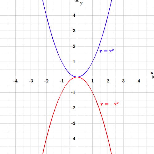 Vertical reflection: The function [latex]y=x^2[/latex] is reflected over the [latex]x[/latex]-axis.
Horizontal Reflections
A horizontal reflection is a reflection across the [latex]y[/latex]-axis, given by the equation: [latex]\displaystyle y=f(-x)[/latex] In this general equation, all [latex]x[/latex] values are switched to their negative counterparts while the y values remain the same. The result is that the curve becomes flipped over the [latex]y[/latex]-axis. Consider an example where the original function is: [latex]\displaystyle y = (x-2)^2[/latex] Therefore the horizontal reflection produces the equation: [latex]\displaystyle \begin{align} y &= f(-x)\\ &= (-x-2)^2 \end{align}[/latex]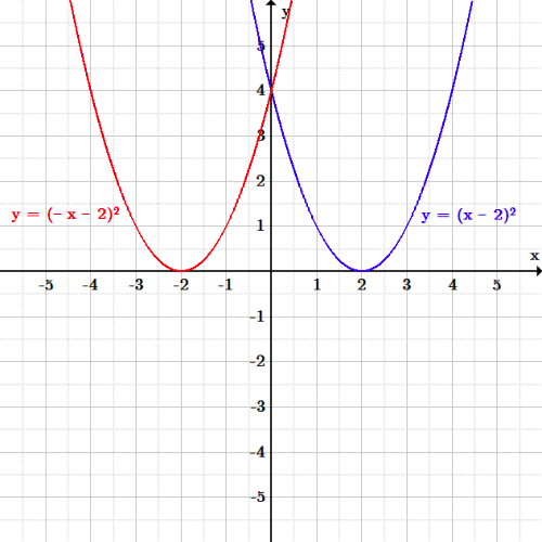 Horizontal reflection: The function [latex]y=(x-2)^2[/latex] is reflected over the [latex]y[/latex]-axis.
Reflections Across a Line
The third type of reflection is a reflection across a line. Let's look at the case involving the line [latex]y=x[/latex]. This reflection has the effect of swapping the variables [latex]x[/latex]and [latex]y[/latex], which is exactly like the case of an inverse function. As an example, let the original function be: [latex]\displaystyle y = x^2[/latex] The reflected equation, as reflected across the line [latex]y=x[/latex], would then be: [latex-display]y = \pm \sqrt{x}[/latex-display]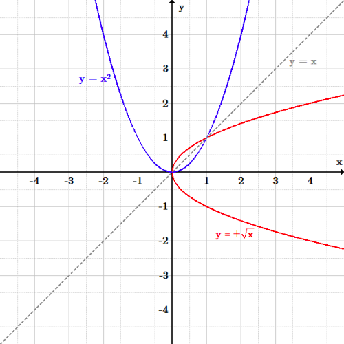 Reflection over [latex]y=x[/latex]: The function [latex]y=x^2[/latex] is reflected over the line [latex]y=x[/latex].
Stretching and Shrinking
Stretching and shrinking refer to transformations that alter how compact a function looks in the [latex]x[/latex] or [latex]y[/latex] direction.Learning Objectives
Manipulate functions so that they stretch or shrink.Key Takeaways
Key Points
- When by either [latex]f(x)[/latex] or [latex]x[/latex] is multiplied by a number, functions can "stretch" or "shrink" vertically or horizontally, respectively, when graphed.
- In general, a vertical stretch is given by the equation [latex]y=bf(x)[/latex]. If [latex]b>1[/latex], the graph stretches with respect to the [latex]y[/latex]-axis, or vertically. If [latex]b<1[/latex], the graph shrinks with respect to the [latex]y[/latex]-axis.
- In general, a horizontal stretch is given by the equation [latex]y = f(cx)[/latex]. If [latex]c>1[/latex], the graph shrinks with respect to the [latex]x[/latex]-axis, or horizontally. If [latex]c<1[/latex], the graph stretches with respect to the [latex]x[/latex]-axis.
Key Terms
- scaling: A transformation that changes the size and/or shape of the graph of the function.
Vertical Scaling
First, let's talk about vertical scaling. Multiplying the entire function [latex]f(x)[/latex] by a constant greater than one causes all the [latex]y[/latex] values of an equation to increase. This leads to a "stretched" appearance in the vertical direction. If the function [latex]f(x)[/latex] is multiplied by a value less than one, all the [latex]y[/latex] values of the equation will decrease, leading to a "shrunken" appearance in the vertical direction. In general, the equation for vertical scaling is: [latex]\displaystyle y = bf(x)[/latex] where [latex]f(x)[/latex] is some function and [latex]b[/latex] is an arbitrary constant. If [latex]b[/latex] is greater than one the function will undergo vertical stretching, and if [latex]b[/latex] is less than one the function will undergo vertical shrinking. As an example, consider the initial sinusoidal function presented below: [latex]\displaystyle y = \sin(x)[/latex] If we want to vertically stretch the function by a factor of three, then the new function becomes: [latex]\displaystyle \begin{align} y &= 3f(x) \\ &= 3\sin(x) \end{align}[/latex]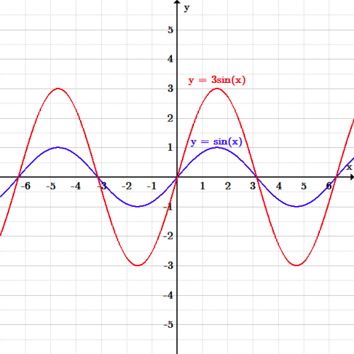 Vertical scaling: The function [latex]y=\sin(x)[/latex] is stretched by a factor of three in the [latex]y[/latex] direction.
Horizontal Scaling
Now lets analyze horizontal scaling. Multiplying the independent variable [latex]x[/latex] by a constant greater than one causes all the [latex]x[/latex] values of an equation to increase. This leads to a "shrunken" appearance in the horizontal direction. If the independent variable [latex]x[/latex] is multiplied by a value less than one, all the x values of the equation will decrease, leading to a "stretched" appearance in the horizontal direction. In general, the equation for horizontal scaling is: [latex]\displaystyle y = f(cx)[/latex] where [latex]f(x)[/latex] is some function and [latex]c[/latex] is an arbitrary constant. If [latex]c[/latex] is greater than one the function will undergo horizontal shrinking, and if [latex]c[/latex] is less than one the function will undergo horizontal stretching. As an example, consider again the initial sinusoidal function: [latex]\displaystyle y = \sin(x)[/latex] If we want to induce horizontal shrinking, the new function becomes: [latex]\displaystyle \begin{align} y &= f(3x)\\ &= \sin(3x) \end{align}[/latex]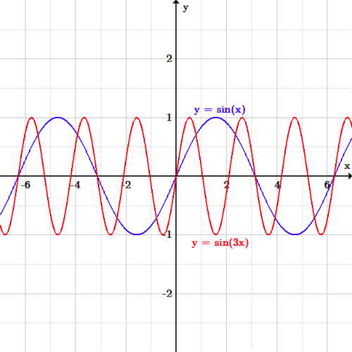 Horizontal scaling: The function [latex]y=\sin(x)[/latex] is shrunk by a factor of three in the [latex]x[/latex] direction.
Licenses & Attributions
CC licensed content, Shared previously
- Curation and Revision. Authored by: Boundless.com. License: Public Domain: No Known Copyright.
CC licensed content, Specific attribution
- Rotation of a Function. Provided by: YouTube License: Public Domain: No Known Copyright.
- Transformations - IB Math Stuff. Provided by: Wikidot Located at: http://ibmathstuff.wikidot.com/transformations. License: CC BY-SA: Attribution-ShareAlike.
- Transformation (function). Provided by: Wikipedia Located at: https://en.wikipedia.org/wiki/Transformation_(function). License: CC BY-SA: Attribution-ShareAlike.
- Original figure by Julien Coyne. Licensed CC BY-SA 4.0. Provided by: Julien Coyne License: CC BY-SA: Attribution-ShareAlike.
- Original figure by Julien Coyne. Licensed CC BY-SA 4.0. Provided by: Julien Coyne License: CC BY-SA: Attribution-ShareAlike.
- Original figure by Julien Coyne. Licensed CC BY-SA 4.0. Provided by: Julien Coyne License: CC BY-SA: Attribution-ShareAlike.
- Algebra/Absolute Value. Provided by: Wikibooks License: CC BY-SA: Attribution-ShareAlike.
- Translation (geometry). Provided by: Wikipedia License: CC BY-SA: Attribution-ShareAlike.
- Transformations - IB Math Stuff. Provided by: Wikidot Located at: http://ibmathstuff.wikidot.com/transformations. License: CC BY-SA: Attribution-ShareAlike.
- vector. Provided by: Wiktionary License: CC BY-SA: Attribution-ShareAlike.
- Original figure by Julien Coyne. Licensed CC BY-SA 4.0. Provided by: Julien Coyne License: CC BY-SA: Attribution-ShareAlike.
- Original figure by Julien Coyne. Licensed CC BY-SA 4.0. Provided by: Julien Coyne License: CC BY-SA: Attribution-ShareAlike.
- Original figure by Julien Coyne. Licensed CC BY-SA 4.0. Provided by: Julien Coyne License: CC BY-SA: Attribution-ShareAlike.
- Original figure by Julien Coyne. Licensed CC BY-SA 4.0. Provided by: Julien Coyne License: CC BY-SA: Attribution-ShareAlike.
- Original figure by Julien Coyne. Licensed CC BY-SA 4.0. Provided by: Julien Coyne License: CC BY-SA: Attribution-ShareAlike.
- Transformations - IB Math Stuff. Provided by: Wikidot Located at: http://ibmathstuff.wikidot.com/transformations. License: CC BY-SA: Attribution-ShareAlike.
- Reflection (mathematics). Provided by: Wikipedia License: CC BY-SA: Attribution-ShareAlike.
- reflection. Provided by: Wiktionary License: CC BY-SA: Attribution-ShareAlike.
- transformation. Provided by: Wiktionary License: CC BY-SA: Attribution-ShareAlike.
- Original figure by Julien Coyne. Licensed CC BY-SA 4.0. Provided by: Julien Coyne License: CC BY-SA: Attribution-ShareAlike.
- Original figure by Julien Coyne. Licensed CC BY-SA 4.0. Provided by: Julien Coyne License: CC BY-SA: Attribution-ShareAlike.
- Original figure by Julien Coyne. Licensed CC BY-SA 4.0. Provided by: Julien Coyne License: CC BY-SA: Attribution-ShareAlike.
- Original figure by Julien Coyne. Licensed CC BY-SA 4.0. Provided by: Julien Coyne License: CC BY-SA: Attribution-ShareAlike.
- Original figure by Julien Coyne. Licensed CC BY-SA 4.0. Provided by: Julien Coyne License: CC BY-SA: Attribution-ShareAlike.
- Original figure by Julien Coyne. Licensed CC BY-SA 4.0. Provided by: Julien Coyne License: CC BY-SA: Attribution-ShareAlike.
- Original figure by Julien Coyne. Licensed CC BY-SA 4.0. Provided by: Julien Coyne License: CC BY-SA: Attribution-ShareAlike.
- Original figure by Julien Coyne. Licensed CC BY-SA 4.0. Provided by: Julien Coyne License: CC BY-SA: Attribution-ShareAlike.
- Transformations - IB Math Stuff. Provided by: Wikidot Located at: http://ibmathstuff.wikidot.com/transformations. License: CC BY-SA: Attribution-ShareAlike.
- Original figure by Julien Coyne. Licensed CC BY-SA 4.0. Provided by: Julien Coyne License: CC BY-SA: Attribution-ShareAlike.
- Original figure by Julien Coyne. Licensed CC BY-SA 4.0. Provided by: Julien Coyne License: CC BY-SA: Attribution-ShareAlike.
- Original figure by Julien Coyne. Licensed CC BY-SA 4.0. Provided by: Julien Coyne License: CC BY-SA: Attribution-ShareAlike.
- Original figure by Julien Coyne. Licensed CC BY-SA 4.0. Provided by: Julien Coyne License: CC BY-SA: Attribution-ShareAlike.
- Original figure by Julien Coyne. Licensed CC BY-SA 4.0. Provided by: Julien Coyne License: CC BY-SA: Attribution-ShareAlike.
- Original figure by Julien Coyne. Licensed CC BY-SA 4.0. Provided by: Julien Coyne License: CC BY-SA: Attribution-ShareAlike.
- Original figure by Julien Coyne. Licensed CC BY-SA 4.0. Provided by: Julien Coyne License: CC BY-SA: Attribution-ShareAlike.
- Original figure by Julien Coyne. Licensed CC BY-SA 4.0. Provided by: Julien Coyne License: CC BY-SA: Attribution-ShareAlike.
- Original figure by Julien Coyne. Licensed CC BY-SA 4.0. Provided by: Julien Coyne License: CC BY-SA: Attribution-ShareAlike.
- Original figure by Julien Coyne. Licensed CC BY-SA 4.0. Provided by: Julien Coyne License: CC BY-SA: Attribution-ShareAlike.
