Graphing Polynomial Functions
Basics of Graphing Polynomial Functions
A polynomial function in one real variable can be represented by a graph.Learning Objectives
Discuss the factors that affect the graph of a polynomialKey Takeaways
Key Points
- The graph of the zero polynomial [latex]f(x) = 0[/latex] is the x-axis.
- The graph of a degree 1 polynomial (or linear function ) [latex]f(x) = a_0 + a_1x[/latex], where [latex]a_1 \neq 0[/latex], is a straight line with y-intercept [latex]a_0[/latex] and slope [latex]a_1[/latex].
- The graph of a degree 2 polynomial [latex]f(x) = a_0 + a_1x + a_2x^2[/latex], where [latex]a_2 \neq 0[/latex] is a parabola.
- The graph of any polynomial with degree 2 or greater [latex]f(x) = a_0 + a_1x + a_2x^2 +... + a_nx^n[/latex], where [latex]a_n \neq 0[/latex] and [latex]n \geq 2[/latex] is a continuous non-linear curve.
Key Terms
- polynomial: an expression consisting of a sum of a finite number of terms, each term being the product of a constant coefficient and one or more variables raised to a non-negative integer power, such as [latex]a_n x^n + a_{n-1}x^{n-1} +... + a_0 x^0[/latex]. Importantly, because all exponents are positive, it is impossible to divide by x.
- indeterminate: not accurately determined or determinable.
- term: any value (variable or constant) or expression separated from another term by a space or an appropriate character, in an overall expression or table.
Visible Properties of a Polynomial
A typical graph of a polynomial function of degree 3 is the following: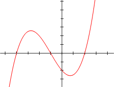 A polynomial of degree [latex]3[/latex]: Graph of a polynomial function with equation [latex]y = \frac {x^3}{4} + \frac {3x^2}{4} - \frac {3x}{2} - 2.[/latex]
Zeros
If we factorize the above function we see that [latex]y = \frac{1}{4}(x-2)(x+1)(x+4)[/latex], so the zeros of the polynomial are [latex]2, -1[/latex] and [latex]-4[/latex]. This is one thing we can read from the graph. In general, we can read the number of zeros from a polynomial just by looking at how many times it meets the [latex]x[/latex]-axis.Behavior Near Infinity
As [latex]\frac {x^3}{4}[/latex] tends to be much larger (in absolute value) than [latex]\frac {3x^2}{4} - \frac {3x}{2} - 2[/latex] when [latex]x[/latex] tends to positive or negative infinity, we see that [latex]y[/latex] goes, like [latex]\frac {x^3}{4}[/latex], to negative infinity when [latex]x[/latex] goes to negative infinity, and to positive infinity when [latex]x[/latex] goes to positive infinity. This is again something we can read from the graph. In general, polynomials will show the same behavior as their highest-degree term. Functions of even degree will go to positive or negative infinity (depending on the sign of the coefficient of the highest-degree term) if [latex]x[/latex] goes to infinity. Functions of odd degree will go to negative or positive infinity when [latex]x[/latex] goes to negative infinity and vice versa, again depending on the highest-degree term coefficient.How to Sketch a Graph
Conversely, if we know the zeros of a polynomial, and we know how it behaves near infinity, we can already make a nice sketch of the graph. We can exactly draw the points [latex](z,0)[/latex] for each root [latex]z[/latex]. Between two zeros (and before the smallest zero, and after the greatest zero) a function will always be either positive, or negative. We know whether it is positive or negative at infinity. Every time we cross a zero of odd multiplicity (if the number of zeros equals the degree of the polynomial, all zeros have multiplicity one and thus odd multiplicity) we change sign. So in our example, we start with a negative sign until we reach [latex]x = -4[/latex], when our graph rises above the [latex]x[/latex]-axis. At some point it starts to descend again, until we reach [latex]x=-1[/latex] and the graph goes below the [latex]x[/latex]-axis again till [latex]x=2[/latex], where it becomes positive again. With this procedure, we can draw a reasonable sketch of our graph, by only looking at the sign of the function and drawing a smooth line with the same sign! However, we can do better. For example, the number of times a function reaches a local minimum or maximum (i.e. a point where the graph descends and then starts to ascend again, or vice versa) is finite. In particular, it is smaller than the degree of the given polynomial. So if you draw a graph, make sure you draw no more local extremum points than you should.Easy Points to Draw
Another easy point to draw is the intersection with the [latex]y[/latex]-axis, as this equals the function value in the point zero, which equals the constant term of the polynomial. We also call this the [latex]y[/latex]-intercept of the function. So if we draw our smooth line, we make sure it crosses the [latex]y[/latex]-axis in the same place. In general, the more function values we compute, the more points of the graph we know, and the more accurate our graph will be. Conversely, we can easily read the constant term of the polynomial by looking at its intersection with the [latex]y[/latex]-axis if its graph is given (and indeed, we can readily read any function value if the graph is given).Examples
- The graph of the zero polynomial [latex]f(x)=0[/latex] is the [latex]x[/latex]-axis, since all real numbers are zeros.
- The graph of a degree [latex]0[/latex] polynomial [latex]f(x)=a_0[/latex], where [latex]a_0 \not = 0[/latex], is a horizontal line with [latex]y[/latex]-intercept [latex]a_0[/latex].
- The graph of a degree 1 polynomial (or linear function)[latex]f(x) = a_0 + a_1x[/latex], where [latex]a_1 \not = 0[/latex], is a straight line with [latex]y[/latex]-intercept [latex]a_0[/latex] and slope [latex]a_1[/latex].
- The graph of a degree 2 polynomial [latex]f(x) = a_0 + a_1x + a_2x^2[/latex], where [latex]a_2 \neq 0[/latex] is a parabola.
- The graph of a degree 3 polynomial [latex]f(x) = a_0 + a_1x + a_2x^2 + a_3x^3[/latex], where [latex]a_3 \neq 0[/latex], is a cubic curve.
- The graph of any polynomial with degree 2 or greater [latex]f(x) = a_0 + a_1x + a_2x^2 +... + a_nx^n[/latex], where [latex]a_n \neq 0[/latex] and [latex]n \geq 2[/latex] is a continuous non-linear curve.
- The graph of a non-constant (univariate) polynomial always tends to infinity when the variable increases indefinitely (in absolute value).
Examples
Below are some examples of graphs of functions.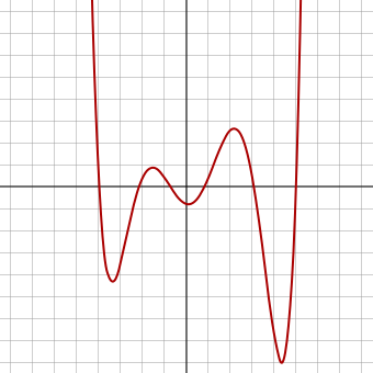 A polynomial of degree 6: A polynomial of degree 6. Its constant term is between -1 and 0. Its highest-degree coefficient is positive. It has exactly 6 zeroes and 5 local extrema.
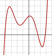 A polynomial of degree 5: A polynomial of degree 5. Its constant term is between 3 and 4. Its highest-degree coefficient is positive. It has 3 real zeros (and two complex ones). However, it has 4 local extrema.
The Leading-Term Test
Analysis of a polynomial reveals whether the function will increase or decrease as [latex]x[/latex] approaches positive and negative infinity.Learning Objectives
Use the leading-term test to describe the end behavior of a polynomial graphKey Takeaways
Key Points
- Properties of the leading term of a polynomial reveal whether the function increases or decreases continually as [latex]x[/latex] values approach positive and negative infinity.
- If [latex]n[/latex] is odd and [latex]a_n[/latex] is positive, the function declines to the left and inclines to the right.
- If [latex]n[/latex] is odd and [latex]a_n[/latex] is negative, the function inclines to the left and declines to the right.
- If [latex]n[/latex] is even and [latex]a_n[/latex] is positive, the function inclines both to the left and to the right.
- If [latex]n[/latex] is even and [latex]a_n[/latex] is negative, the function declines both to the left and to the right.
Key Terms
- Leading term: The term in a polynomial in which the independent variable is raised to the highest power.
- Leading coefficient: The coefficient of the leading term.
Leading Term, Leading Coefficient and Leading Test
All polynomial functions of first or higher order either increase or decrease indefinitely as [latex]x[/latex] values grow larger and smaller. It is possible to determine the end behavior (i.e. the behavior when [latex]x[/latex] tends to infinity) of a polynomial function without using a graph. Consider the polynomial function: [latex-display]f(x)=a_nx^n + a_{n-1}x^{n-1}+...+a_1x+a_0[/latex-display] [latex]a_nx^n[/latex] is called the leading term of [latex]f(x)[/latex], while [latex]a_n \not = 0[/latex] is known as the leading coefficient. The properties of the leading term and leading coefficient indicate whether [latex]f(x)[/latex] increases or decreases continually as the [latex]x[/latex]-values approach positive and negative infinity:- If [latex]n[/latex] is odd and [latex]a_n[/latex] is positive, the function declines to the left and inclines to the right.
- If [latex]n[/latex] is odd and [latex]a_n[/latex] is negative, the function inclines to the left and declines to the right.
- If [latex]n[/latex] is even and [latex]a_n[/latex] is positive, the function inclines both to the left and to the right.
- If [latex]n[/latex] is even and [latex]a_n[/latex] is negative, the function declines both to the left and to the right.
Examples
Consider the polynomial [latex-display]f(x) = \frac {x^3}{4} + \frac {3x^2}{4} - \frac {3x}{2} -2.[/latex-display] In the leading term, [latex]a_n[/latex] equals [latex]\frac {1}{4}[/latex] and [latex]n[/latex] equals [latex]3[/latex]. Because [latex]n[/latex] is odd and [latex]a[/latex] is positive, the graph declines to the left and inclines to the right. This can be seen on its graph below: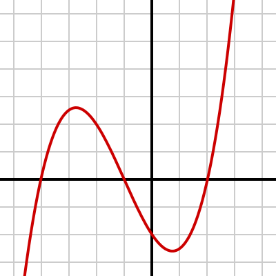 A polynomial of degree [latex]3[/latex]: Graph of a polynomial with equation [latex]f(x) = \frac {x^3}{4} + \frac {3x^2}{4} - \frac{3x}{2} - 2[/latex]. Because the degree is odd and the leading coefficient is positive, the function declines to the left and inclines to the right.
Another example is the function
[latex-display]g(x) = - \frac{1}{14} (x+4)(x+1)(x-1)(x-3) + \frac{1}{2}[/latex-display] which has [latex]-\frac {x^4}{14}[/latex] as its leading term and [latex]- \frac{1}{14}[/latex] as its leading coefficient. Thus [latex]g(x)[/latex]approaches negative infinity as [latex]x[/latex] approaches either positive or negative infinity; the graph declines both to the left and to the right as seen in the next figure: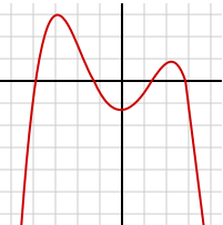 A polynomial of degree 4: Graph of [latex]g(x) = - \frac{1}{14} (x+4)(x+1)(x-1)(x-3) + \frac{1}{2}[/latex]. As the degree is even and the leading coefficient is negative, the function declines both to the left and to the right.
The Leading Test Explained
Intuitively, one can see why we need to look at the leading coefficient to see how a polynomial behaves at infinity: When [latex]x[/latex] is very big (in absolute value ), then the highest degree term will be much bigger (in absolute value) than the other terms combined. For example [latex]x - 1000[/latex] differs a lot from [latex]x[/latex] when [latex]x = 0[/latex] or [latex]1000[/latex], but (relatively) not when [latex]x = 9999999999999[/latex] or [latex]-9999999999999999[/latex]. Indeed, both functions can be described as "very big and positive" in the first point and "very big and negative" in the second. In general, when we have a polynomial [latex-display]f(x) = a_nx^n + \ldots + a_0[/latex-display] and the absolute value of [latex]x[/latex] is bigger than [latex]MnK[/latex], where [latex]M[/latex] is the absolute value of the largest coefficient divided by the leading coefficient, [latex]n[/latex] is the degree of the polynomial and [latex]K[/latex] is a big number, then the absolute value of [latex]a_nx^n[/latex] will be bigger than [latex]nK[/latex] times the absolute value of any other term, and bigger than [latex]K[/latex] times the other terms combined! So when [latex]x[/latex] grows very large, [latex]f(x)[/latex] very much resembles its leading term [latex]a_n x^n.[/latex] This function grows very big as [latex]x[/latex] grows very big. Now [latex]a_nx^n[/latex] takes on the sign of [latex]a_n[/latex] if [latex]x^n[/latex] is positive, which happens if [latex]x[/latex] is positive or if [latex]n[/latex] is even, and the opposite sign of [latex]a_n[/latex] if [latex]x^n[/latex] is negative, which happens if [latex]x[/latex] is negative and [latex]n[/latex] is odd. (Notice that we do not care about [latex]x = 0[/latex] since we are only interested in very large [latex]x.[/latex]) Thus, [latex]a_nx^n[/latex] (and thus [latex]f(x)[/latex], in the neighborhood of infinity) goes up (as [latex]x[/latex] approaches infinity) if [latex]a^n[/latex] is positive and down if [latex]a_n[/latex] is negative. Except when [latex]x[/latex] is negative and [latex]n[/latex] is odd; then the opposite is true.Licenses & Attributions
CC licensed content, Shared previously
- Curation and Revision. Authored by: Boundless.com. License: Public Domain: No Known Copyright.
CC licensed content, Specific attribution
- Polynomial. Provided by: Wikipedia Located at: https://en.wikipedia.org/wiki/Polynomial. License: CC BY-SA: Attribution-ShareAlike.
- term. Provided by: Wiktionary License: CC BY-SA: Attribution-ShareAlike.
- indeterminate. Provided by: Wiktionary License: CC BY-SA: Attribution-ShareAlike.
- polynomial. Provided by: Wiktionary License: CC BY-SA: Attribution-ShareAlike.
- 180px-Quintic_polynomial.svg.png. Provided by: Quintic polynomial Located at: https://upload.wikimedia.org/wikipedia/commons/thumb/8/8a/Quintic_polynomial.svg/180px-Quintic_polynomial.svg.png. License: CC BY-SA: Attribution-ShareAlike.
- Sextic_Graph.svg. Provided by: A polynomial of degree 6 Located at: https://upload.wikimedia.org/wikipedia/commons/c/c3/Sextic_Graph.svg. License: CC BY-SA: Attribution-ShareAlike.
- Polynomialdeg3.png. Provided by: Wikipedia License: CC BY-SA: Attribution-ShareAlike.
- Coefficient. Provided by: Wikipedia License: CC BY-SA: Attribution-ShareAlike.
- Leading term. Provided by: Wikipedia License: CC BY-SA: Attribution-ShareAlike.
- Boundless. Provided by: Boundless Learning License: CC BY-SA: Attribution-ShareAlike.
- 180px-Quintic_polynomial.svg.png. Provided by: Quintic polynomial Located at: https://upload.wikimedia.org/wikipedia/commons/thumb/8/8a/Quintic_polynomial.svg/180px-Quintic_polynomial.svg.png. License: CC BY-SA: Attribution-ShareAlike.
- Sextic_Graph.svg. Provided by: A polynomial of degree 6 Located at: https://upload.wikimedia.org/wikipedia/commons/c/c3/Sextic_Graph.svg. License: CC BY-SA: Attribution-ShareAlike.
- Polynomialdeg3.png. Provided by: Wikipedia Located at: https://en.wikipedia.org/wiki/Polynomial. License: CC BY-SA: Attribution-ShareAlike.
- Boundlessminusminus.png. Provided by: Wikipedia License: CC BY-SA: Attribution-ShareAlike.
- 400px-Polynomialdeg3.svg.png. Provided by: Wikipedia Located at: https://upload.wikimedia.org/wikipedia/commons/thumb/a/a3/Polynomialdeg3.svg/400px-Polynomialdeg3.svg.png. License: CC BY-SA: Attribution-ShareAlike.
