Applications of Exponential and Logarithmic Functions
Population Growth
Population can fluctuate positively or negatively and can be modeled using an exponential function.
Learning Objectives
Use exponential functions to represent population growth
Key Takeaways
Key Points
- The formula for population growth is [latex]P(r,t,f)=P{_i}(1+r)^{\frac{t}{f}}[/latex] where [latex]P{_i}[/latex] represents initial population, [latex]r[/latex] is the rate of population growth (expressed as a decimal), [latex]t[/latex] is elapsed time, and [latex]f[/latex] is the period over which time population grows by a rate of [latex]r[/latex].
- Population growth is dependent on four variables: Births ([latex]B[/latex] ), deaths ([latex]D[/latex]), immigrants ([latex]I[/latex]), and emigrants ([latex]E[/latex] ). Using these we model population growth as [latex]{\Delta}P=(B-D)+(I-E)[/latex] where [latex]{\Delta}P[/latex] is the change in population.
- Population growth rate can reveal whether a population size is increasing (positive) or decreasing (negative). It can be calculated for two distinct times with the following equation: [latex]PGR=\frac{ln(P(t_2))-ln(P(t_1))}{(t_2-t_1)}[/latex] where [latex]t{_2}[/latex] and [latex]t{_1}[/latex] are the two distinct times.
Key Terms
- exponential: Any function that has an exponent as an independent variable.
- emigrant: Someone who leaves a country to settle in a new country.
- immigrant: A person who comes to a country from another country in order to permanently settle in the new country.
Introduction
Population growth can be modeled by an exponential equation. Namely, it is given by the formula [latex]P(r, t, f)=P_i(1+r)^\frac{t}{f}[/latex] where [latex]P{_i}[/latex] represents the initial population, r is the rate of population growth (expressed as a decimal), t is elapsed time, and f is the period over which time population grows by a rate of r. The ratio of t to f is often simplified into one value representing the number of compounding cycles.
The rate [latex]r[/latex] by which the population is growing is itself a function of four variables. These are births ([latex]B[/latex] ), deaths ([latex]D[/latex]), immigrants ([latex]I[/latex]) and emigrants ([latex]E[/latex]). Specifically, the rate is given by:
[latex-display]{\Delta}P=(B-D)+(I-E)[/latex-display]
[latex]{\Delta}P[/latex] denotes the change in population. The formula is split into natural growth which accounts for births and deaths ([latex]B-D[/latex]) and mechanical growth which accounts for people moving into and out of a particular region ([latex]I-E[/latex]).
Population Growth Rate
The population size can fluctuate from growth to decline, and back again. As such, another variable is important when studying population demographics and dynamics. It is the Population Growth Rate ([latex]PGR[/latex]).
[latex]PGR[/latex] is the rate of change in population over a certain span of time: [latex]t_2-t_1[/latex]. It can be determined using the formula:
[latex]\displaystyle
PGR=\frac{ln(P(t_2))-ln(P(t_1))}{(t_2-t_1)}[/latex]
If we multiply the [latex]PGR[/latex] by [latex]100[/latex] we arrive at the percentage growth relative to the population at the beginning of the time period.
A positive growth rate indicates an increasing population size, while a negative growth rate is characteristic of a decreasing population. A growth rate of [latex]0[/latex] means stagnation in population size.
World Population
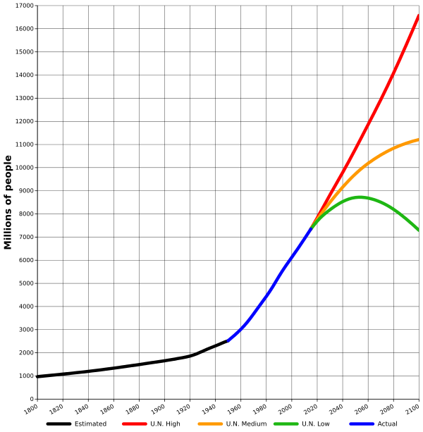
In demographics, the world population is the total number of humans currently living. As of March 2016, it was estimated at 7.4 billion, an all-time high. The United Nations estimates it will further increase to 11.2 billion in the year 2100. If the current rates of births and deaths hold, the world population growth can be modeled using an exponential function. The graph below shows an exponential model for the growth of the world population.
 World-Population from 1800 (actual) to 2100 (projected):
 The projected world population growths after the present day must be projected. A high estimation predicts the graph to continue at an increasing rate, a medium estimation predicts the population to level off, and a low estimation predicts the population to decline.
Limited Growth
A realistic model of exponential growth must dampen when approaching a certain value. This limited growth is modelled with the logistic growth model: [latex]P(t)=\frac{c}{1+a\cdot e^{-bt}}[/latex].
Learning Objectives
Use logistic functions to represent limited growth
Key Takeaways
Key Points
- Exponential growth may exist within known parameters, but such a functionality may not continue indefinitely in the real world.
- If a natural maximum is conceivable, the logistic growth model can be used to represent growth. It has the form: [latex]P(t)=\frac{c}{1+a\cdot e^{-bt}}[/latex]where [latex]P[/latex] represents population, [latex]c[/latex] is the carrying capacity, [latex]b[/latex] is the population growth rate, [latex]t[/latex] is time, and [latex]a[/latex] is the difference between carrying capacity and initial population.
- An example of natural dampening in growth is the population of humans on planet Earth. The population may be growing exponentially at the moment, but eventually, scarcity of resources will curb our growth as we reach our carrying capacity.
Key Terms
- logistic function: A defined function that is the result of the division of two exponential functions. When plotted it gives the logistic curve.
Introduction
Exponential functions can be used to model growth and decay. For example, the world's human population is growing exponentially as can be seen in the following graph.
 World Population from 1800 AD to 2100 AD:
 Three projections for the world's population are shown, with a low estimate reaching a peak and then decreasing, a medium estimate increasing but at an ever-slower rate, and a high estimate continuing to increase exponentially.
Logistic Growth Model
To account for limitations in growth, the logistic growth model can be used. The logistic growth model is given by [latex]P(t)=\frac{c}{1+a\cdot e^{-bt}}[/latex] where [latex]P[/latex] represents the present population, [latex]c[/latex] is the carrying capacity (the maximum the population approaches as time approaches infinity), [latex]b[/latex] is the population growth rate, [latex]t[/latex] is time, and [latex]a[/latex] is the difference between carrying capacity and initial population.
Evaluating a Logistic Growth Function
Given various conditions, it is possible to evaluate a logistic function for a particular value of [latex]t[/latex]. That is, it is possible to determine the population at time [latex]t[/latex], given values for [latex]c,a,b[/latex] and [latex]t[/latex].
Example 1: Evaluate the logistic growth function [latex]P(t)=\frac{50}{1+8\cdot e^{-3t}}[/latex] for [latex]t=6[/latex]
To evaluate this function we plug [latex]6[/latex] into the equation in place of [latex]t[/latex] as follows.
[latex]\displaystyle
\begin{align}
P(6)&=\frac{50}{1+8\cdot e^{(-3)(6)}}\\&
\approx49.99999391
\end{align}[/latex]
Graphing a Logistic Growth Model
Graphically, the logistic function resembles an exponential function followed by a logarithmic function that approaches a horizontal asymptote. This horizontal asymptote represents the carrying capacity. That is, [latex]y=c[/latex] is a horizontal asymptote of the graph. Additionally, [latex]y=o[/latex] is also a horizontal asymptote. From the left, it grows rapidly, but that growth is dampened as time passes to where it reaches a maximum. The function's domain is the set of all real numbers, whereas its range is [latex]0<y<c[/latex]. Below is the graph of a logistic function.
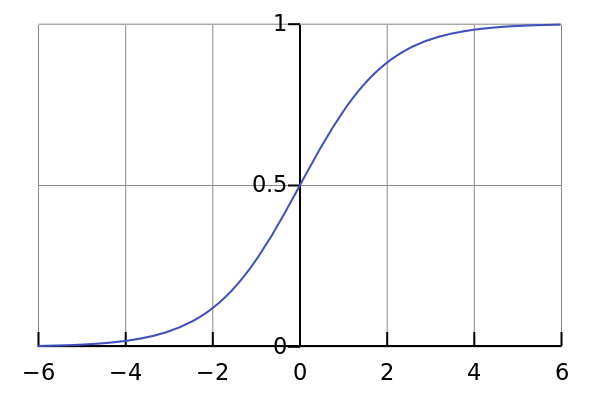 Graph of a logistic function:
 Logistic functions have an "s" shape, where the function starts from a certain point, increases, and then approaches an upper asymptote.
Interest Compounded Continuously
Compound interest is accrued when interest is earned not only on principal, but on previously accrued interest: it is interest on interest.
Learning Objectives
Differentiate between simple interest and compound interest
Key Takeaways
Key Points
- Interest is, generally, a fee charged for the borrowing of money. The amount of interest accrued depends on the principal (amount borrowed), the interest rate (a percentage of the principal), period (amount of time between interest payments) and time elapsed.
- The form of the equation for compound interest is exponential, and thus such interest is accrued much faster than the linear simple interest.
- The formula for compound interest is [latex]M=p(1+r)^\frac{t}{f}[/latex]Where [latex]M[/latex] represents the total value (including principal), [latex]p[/latex] represents principal, [latex]r[/latex] is interest rate (expressed as a decimal), [latex]t[/latex] is time elapsed, and [latex]f[/latex] is the length of time between payments. To calculate interest alone, simply subtract the principal from [latex]M[/latex].
Key Terms
- exponential function: Any function in which an independent variable is in the form of an exponent; they are the inverse functions of logarithms.
- compound interest: Interest, as on a loan or a bank account, that is calculated on the total on the principal plus accumulated unpaid interest.
- Interest: The price paid for obtaining, or price received for providing, money or goods in a credit transaction, calculated as a fraction of the amount or value of what was borrowed.
Introduction
Fundamentally, compound interest is an application of exponential functions that is found very commonly in every day life. Interest is, generally, a fee charged for the borrowing of money. The two classic cases are (1) interest accrued as part of loan and (2) interest accrued in a savings or other account. In the first case the client owes the amount borrowed plus the interest. In the second, the bank pays the client interest for maintaining money in the account. If you are the client, you are losing money in the first case and earning money in the second.
The amount of interest accrued depends on the principal (amount borrowed/deposited), the interest rate (a percentage of the principal), period (amount of time between interest payments) and time elapsed.
For questions of interest, unless otherwise stated, the amount borrowed/deposited remains unchanged. The client does not, for example, add or withdraw funds from the savings account after the initial deposit (the principal) is made.
Simple vs. Compound Interest
There exist two kinds of interest: simple and compound.
In simple interest, interest is accrued on the principal alone. This means that the amount of interest earned in each compounding period is the same because interest is earned based on the principal which remains unchanged.
In compound interest, interest is accrued on both the principal and on prior interest earned. For this reason, if all other conditions are the same (principal, rate, time elapsed and frequency of interest payments) compound interest grows at a faster rate than simple interest. The amount of interest earned increases with each compounding period.
Simple Interest: An Example
Simple interest is accrued linearly based on the formula:
[latex]\displaystyle
I=p\cdot r \cdot \frac{t}{f}[/latex]
Where [latex]I[/latex] represents the interest, [latex]p[/latex] is the principal, [latex]r[/latex] is interest rate (expressed as a decimal), [latex]t[/latex] is time elapsed, and [latex]f[/latex] is the time elapsed per interest payment. The ratio of [latex]t[/latex] to [latex]f[/latex] is often simplified to the number of interest payments. Total amount owed/earned which includes the principal and the interest is given by [latex]A=P+I[/latex].
Example 1: You deposit $100 into a bank account earning 5% annual interest. How much money is in the account at the end of 1, 2, 3, 4, and [latex]n[/latex]years?
Let us begin by determining the interest at the end of the first year. We use the formula [latex]I=p\cdot r \cdot \frac{t}{f}[/latex] with [latex]p=100[/latex], [latex]r=.05[/latex], [latex]t=1[/latex] and [latex]f=1[/latex]. The interest earned at the end of the year is:
[latex]\displaystyle
\begin{align}
I&=(100)(.05)(\frac{1}{1})\\&
=5
\end{align}[/latex]
The amount in the account at the conclusion of the year is given by [latex]100+5=105[/latex]. It is useful to note that the account will earn $[latex]5[/latex] in interest every single year irrespective of how long the money is in the account or what the amount in the account is during any given year. This can be seen by the fact that the amount after [latex]n[/latex] years is given by a linear function with slope equal to five (see table below).
The table below shows the calculations, interest earned and total amount in the account after 1, 2, 3, 4, and n years.
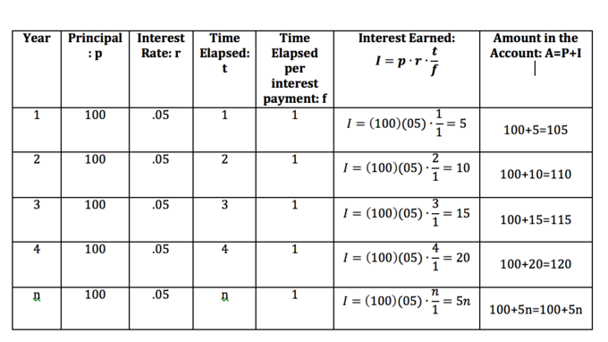 Calculations of interest earned and amount in the account for Example 1
Compound Interest: An Example
Compound interest is not linear, but exponential in form. That is, the amount of interest earned is not constant but instead changes with time based on the total amount of the amount in the account.
The equation representing investment value as a function of principal, interest rate, period and time is:
[latex]\displaystyle
M=p(1+r)^\frac{t}{f}[/latex]
Where [latex]M[/latex] represents the total value (including principal), [latex]p[/latex] represents principal, [latex]r[/latex] is interest rate (expressed as a decimal), [latex]t[/latex] is time elapsed, and [latex]f[/latex] is the length of time between payments. To calculate interest alone, simply subtract the principal from [latex]M[/latex].
We now re-consider Example 1 above. This time we use compound interest instead.
Example
2: You deposit $100 into a bank account earning 5% interest compounded annually. How
much money is in the account at the end of 1, 2, 3, 4, and [latex]n[/latex] years?
Let us begin by determining the amount in the account after the first year using the formula [latex]M=p(1+r)^\frac{t}{f}[/latex] with [latex]p=100[/latex], [latex]r=.05[/latex], [latex]t=1[/latex] and [latex]f=1[/latex]. The amount in the account after one year is:
[latex]\displaystyle
\begin{align}
M&=(100)(1+.05)^\frac{1}{1}\\
&=105
\end{align}[/latex]
This is the exact amount that was in the account after the first year using simple interest. That is because the difference is that compound interest earns interest on both the principal and prior interest. At the end of the first year there was no prior interest in the account. We will see differences between simple and compound interest in this, and similar problems, in the second year.
Let us determine the amount in the account after the second year again using the formula [latex]M=p(1+r)^\frac{t}{f}[/latex] but now letting [latex]t=2[/latex]. We obtain:
[latex]\displaystyle
\begin{align}
M&=100(1+.05)^\frac{2}{1}\\
&=110.25
\end{align}[/latex]
That is, there are [latex]25[/latex] cents more in account in the second year using compound interest instead of simple interest. This might not seem like a lot but the amount of interest earned will continue to increase each year as there is more and more money in the account. Every year the interest earned will be higher than in the previous year, whereas in simple interest the amount each year is fixed.
The following table includes the calculations, interest earned and total amount in the account at the end of [latex]1,2,3,4[/latex] and [latex]n[/latex] years.
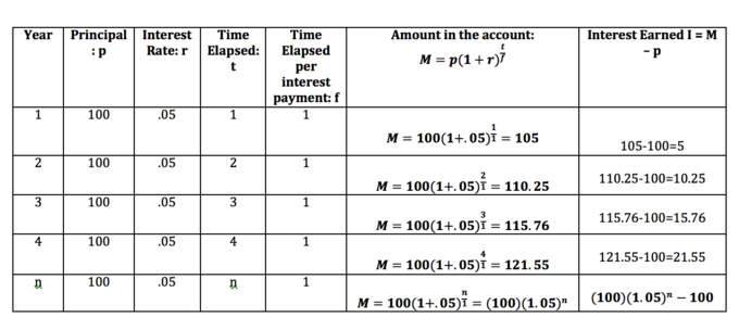
Calculations of interest earned and amount in the account for Example 2
Simple vs. Compound Interest Over Time: An Example
The biggest differences between the amount of money in an account using simple versus compound interest are seen over extended periods of time. To highlight this, we return the the examples we did prior and now consider how much money is in each account after 50 years.
Example
3: You deposit $100 into a bank account earning 5% interest compounded annually. How
much money is in the account at the end of 50 years? How does this compare to the amount in the account after 50 years if the interest had been compounded annually?
The money in the account using simple interest after [latex]50[/latex] years is given by
[latex]\displaystyle
\begin{align}
P+I&=100+(100)(.05)(\frac{50}{1})\\
&=350
\end{align}[/latex]
However, the amount in the account using compound interest after [latex]50[/latex] years is given by:
[latex]\displaystyle
\begin{align}
M&=(100)(1+.05)^\frac{50}{1}\\
&=1146.74
\end{align}[/latex]
A difference of $[latex]796.74[/latex].
Frequency of Compounding Periods
The more frequent the compounding periods the more interest is accrued. Therefore, if one deposits money into a bank account that earns compound interest, and does not add or withdraw any additional funds, the amount of money in the bank would increase as the number of compounding periods per year increases. You earn more interest when interest is compounded quarterly ([latex]4[/latex] times a year) than once a year. You earn more interest when interest is compounded monthly ([latex]12[/latex] times a year) than quarterly. You earn more interest when interest is compounded daily ([latex]365[/latex] times a year) than monthly and so on. You earn the most interest when interest is compounded continuously.
 Graph of interest accrued under differing number of compounding periods per year:
 Starting with a principal of $1000, interest rises exponentially. The graph shows that the more frequent the number of compounding periods the more interest is accrued and shows this visually for yearly, quarterly, monthly and continuous compounding.
Interest Compounded Continuously
Given that the more frequent the compounding periods per year, the more interest is accrued it might come as a surprise that money deposited into a bank account accrues compound interest continuously. You might expect the bank would choose a smaller number of compounding periods in order to pay out less in interest, but this is not the case. To see why let us take the following example: You deposit $[latex]1[/latex] in the bank in an account earning [latex]100[/latex]% interest. You do not add or withdraw money from the account. In this situation the amount of money in the account will be given by [latex](1+\frac{1}{n})^n[/latex] where [latex]n[/latex] is the number of compounding periods and [latex]\frac{1}{n}[/latex] is the rate per compounding period. This is a simplification of the prior formula used because of the specific conditions of this most recent situation. We expect that as [latex]n[/latex] increases the amount in the account also increases, but if the amount grows without bounds then banks would be giving away much money as they compound interest continuously.
The following table shows the amount in the account at the end of one year when interest is compounded with differing frequencies.
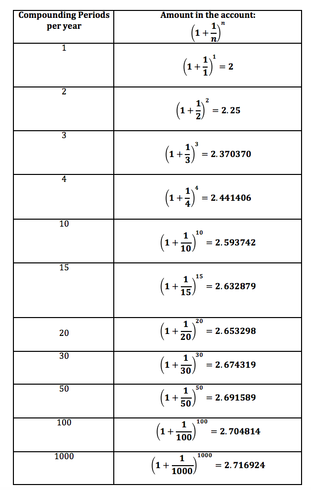 Amount in account after 1 year with interest compounded at different frequencies
Exponential Decay
Exponential decay is the result of a function that decreases in proportion to its current value.
Learning Objectives
Use the exponential decay formula to calculate how much of something is left after a period of time
Key Takeaways
Key Points
- Exponential decrease can be modeled as: [latex]N(t)=N_0e^{-\lambda t}[/latex] where [latex]N[/latex] is the quantity, [latex]N_0[/latex] is the initial quantity, [latex]\lambda[/latex] is the decay constant, and [latex]t[/latex] is time.
- Oftentimes, half-life is used to describe the amount of time required for half of a sample to decay. It can be defined mathematically as: [latex]t_{1/2}=\frac{ln(2)}{\lambda }[/latex]where [latex]t_{1/2}[/latex] is half-life.
- Half-life can be inserted into the exponential decay model as such: [latex]N(t)=N_0(\frac{1}{2})^{t/t_{1/2}}[/latex]. Notice how the exponential changes, but the form of the function remains.
Key Terms
- half-life: The time it takes for a substance (drug, radioactive nuclide, or other) to lose half of its pharmacological, physiological, biological, or radiological activity.
- isotope: Any of two or more forms of an element where the atoms have the same number of protons, but a different number of neutrons. As a consequence, atoms for the same isotope will have the same atomic number but a different mass number (atomic weight).
Introduction
Just as it is possible for a variable to grow exponentially as a function of another, so can the a variable decrease exponentially. Consider the decrease of a population that occurs at a rate proportional to its value. This rate at which the population is decreasing remains constant but as the population is continually decreasing the overall decline becomes less and less steep.
Exponential rate of change can be modeled algebraically by the following formula:
[latex-display]N(t)=N_0e^{-\lambda t}[/latex-display]
where [latex]N[/latex] is the quantity, [latex]N{_0}[/latex] is the initial quantity, [latex]\lambda[/latex] is the decay constant, and [latex]t[/latex] is time. The decay constant is indeed a constant, but the form of the equation (the negative exponent of e) results in an ever-changing rate of decline.
Half Life
The time it takes for a substance (drug, radioactive nuclide, or other) to lose half of its pharmacological, physiological, biological, or radiological activity is called its half-life. The exponential decay of the substance is a time-dependent decline and a prime example of exponential decay.
As an example let us assume we have a [latex]100[/latex] pounds of a substance with a half-life of [latex]5[/latex] years. Then in [latex]5[/latex] years half the amount ([latex]50[/latex] pounds) remains. In another [latex]5[/latex] years there will be [latex]25[/latex] pounds remaining. In another [latex]5[/latex] years, or [latex]15[/latex] years from the beginning, there will be [latex]12.5[/latex]. The amount by which the substance decreases, is itself slowly decreasing.
Use of Half Life in Carbon Dating
Half-life is very useful in determining the age of historical artifacts through a process known as carbon dating. Given a sample of carbon in an ancient, preserved piece of flesh, the age of the sample can be determined based on the percentage of radioactive carbon-13 remaining. 1.1% of carbon is C-13 and it decays to carbon-12. C-13 has a half-life of 5700 years—that is, in 5700 years, half of a sample of C-13 will have converted to C-12, which represents approximately all the remaining carbon. Using this information it is possible to determine the age of the artifact given the amount of C-13 it presently contains, and comparing it to the amount of C-13 it should contain.
Half-life can be mathematically defined as:
[latex]\displaystyle
t_{1/2}=\frac{ln(2)}{\lambda }[/latex]
It can also be conveniently inserted into the exponential decay formula as follows:
[latex]\displaystyle
N(t)=N_0(\frac{1}{2})^{t/t_{1/2}}[/latex]
Thus, if a sample is found to contain 0.55% of its carbon as C-13 (exactly half of the usual 1.1%), it can be calculated that the sample has undergone exactly one half-life, and is thus 5,700 years old.
Below is a graph highlighting exponential decay of a radioactive substance. Using the graph, find that half-life.
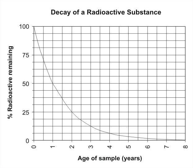 Graph depicting radioactive decay:
 The amount of a substance undergoing radioactive decay decreases exponentially, eventually reaching zero. Since there is 50% of the substance left after 1 year, the half-life is 1 year.
Licenses & Attributions
CC licensed content, Shared previously
CC licensed content, Specific attribution
