Reading: Curve Sketching
Maxima and Minima of Functions
Much can be done to sketch the approximate graph of a function without calculus, in fact I strongly encourage you to rely mostly on your pre-calculus skills to sketch graphs. But by adding the derivative and second derivative to our toolbox, we can determine the exact locations of maxima and minima (collectively "extrema") of a function, and more. First a little terminology:

Figure 1

Figure 2
More Terminology
A global maximum or minimum might sometimes be called "local." Think of it like the Venn diagram in figure 2. Global maxima and minima are a subset of local maxima and minima. On a given interval of the domain of a function, there can be only one global (or absolute) max. and min.—if either exists.
Remember that the derivative, f ′(x), of the function f(x) gives the slope of f(x) at any differentiable point in its domain.
The derivative of a rising function (positive slope) is positive, and the derivative of a falling function (negative slope) is negative.
In the middle case, where the slope is zero, the function graph is neither rising nor falling, but is (usually) a relative maximum or minimum value. Fermat's theorem sums this up:
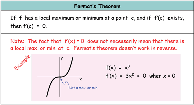
Figure 3
Proof
Referring to the definition of the local maximum above, we see that if a maximum value lies at x = c, then f(x) must be larger than some other value of the function f(x + h), where h can be positive or negative. So: [latex] f(c) \geq f(c + h) [/latex] which rearranges to [latex] f(c + h) - f(c) \leq 0 [/latex]
We can divide both sides of this inequality by h to make this look like a derivative, then take the limit as h → 0+ from the right:
[latex-display] \lim_{h \to 0^+} \frac{f(c+h)-f(c)}{h} = \lim_{h \to 0^+} 0 = 0 [/latex-display]
Now we have assumed that f′(c) exists, so the limit from the right must equal the limit in general:
[latex-display] \lim_{h \to 0^+} \frac{f(c+h)-f(c)}{h} = \lim_{h \to 0} \frac{f(c+h)-f(c)}{h} [/latex-display]
The second equation is f ′(c).
Plugging f ′(c) into the last inequality, we get: f ′(c) ≤ 0
Now we could also do the same proof using the limit from the left, which would lead us to the inequality f ′(c) ≥ 0. The only way that both inequalities can be true is for f ′(c) to be equal to zero, so we have proved Fermat's theorem. Caution: Fermat's theorem doesn't necessarily work both ways.
Go back and look at the Fermat's theorem box above and make sure to understand that the existence of a zero in the derivative function does not guarantee the existence of a relative or global max. or min. there. The graph of y = x3, for example, has a horizontal tangent at x = 0, but it has no maxima or minima at all.
Here's a summary of the relationships of the first derivative of a function to maxima and minima (either local or global) in its graph:

Figure 4
Example 1
Find the x-coordinates of the maxima and minima of f(x) = −x3 + 4x2 + 4x − 16
It's very important when working these problems, not to forget your pre-calculus skills, the algebra skills you learned prior to calculus. Calculus won't replace the skills you already have, it will just enhance what you can learn about the graph of a function. Don't forget your pre-calculus curve-sketching skills. Most of curve sketching does not require (and doesn't benefit from) calculus.
We begin by noting that this function can be factored by grouping:
[latex-display] f(x) = -x(x^2 -4)+ 4(x^2 -4) [/latex-display]
[latex-display] f(x) = (4 -x)(x^2 -4) [/latex-display]
[latex] f(x) = (4 -x)(x + 2)(x - 2) [/latex] Real roots at x 4, ±2
The leading term is negative, so we know this function grows without bound on the left as x → −∞, and tends to −∞ as x → ∞ (i.e. goes up on the left and down on the right). We also know, from our familiarity with the sigmoidal (sideways-S) shape of the graphs of cubic functions, that the left-most extremum (which lies between x = −2 and x = 2, should be the local minimum and the right-most (between x = 2 and x = 4) the maximum. Here's a schematic picture:

Figure 5
| The derivative |
[latex] f\prime(x) = -3x^2 + 8x + 4 [/latex] |
| Set the derivative equal to zero |
[latex] -3x^2 + 8x + 4 = 0 [/latex] |
| Complete the square to find the roots |
[latex] -3x^2 + 8x = -4 [/latex] |
|
[latex] x^2 - \frac{8}{3}x + (\frac{4}{3})^2 = \frac{16}{9} + {12}{9} [/latex] |
|
[latex] (x -\frac{4}{3})^2 = \frac{28}{9} [/latex] |
|
[latex] x = \frac{4 \pm 2 \sqrt7}{3} [/latex] |
| Locations of the extrema |
x ≈ −0.4, 3.1 |

Figure 6
Example 2
A cylindrical metal can is to hold 1 liter of olive oil. Find the dimensions of the can that holds 1 liter and requires the least metal possible to manufacture.

Figure 7
The First Derivative

Figure 8
- If the slope on the left side of an extreme value is negative and that on the right is positive, the extreme value is a minimum.
- If the slope on the left side of an extreme value is positive and that on the right is negative, the extreme value is a maximum.
On both sides of x = 1 the slope of f(x) is negative except at x = 1, where it is zero. That means it can't be a maximum or a minimum (a case where the reverse of Fermat's theorem wouldn't work). The slope of the function must change sign on either side of a maximum or a minimum.
Now compare our function with its second derivative. The second derivative describes the change in the slope of a function—whether the slope of the function is increasing or decreasing. The second derivative couldn't be easier: It's just the derivative of the derivative:
The second derivative of a function is the derivative of its derivative.
[latex-display] f\prime \prime(x) = \frac{d}{dx}(\frac{df}{dx}) = \frac{d^2}{dx^2} f(x) = D_x^2 f(x) [/latex-display]
There is a bit of extra notation there. It's easiest, and very common, to use the compact notation f″(x) for the second derivative. The third notation is a little illogical (we're not taking a derivative with respect to x2, but it's very commonly used, so you should get used to it. The third is due to Euler; it's compact and descriptive, but only used sometimes.

Figure 9
The Second Derivative
The second derivative is a good indicator of the curvature of a function. In this comparison, notice that every zero (f″(x) = 0) in the graph of the second derivative matches an inflection point in the graph of f(x).
The zeros in f′(x) all align with inflection points. In particular, the zero at x = 1 confirms the inflection point we already knew.
It is possible, however, that a zero in the 2nd derivative of a function does not indicate an inflection point. For example, the function g(x) = x4 has a zero at x = 0 in its second derivative, g″(x) = 12x2, but that point is actually the global minimum of that function, with concave-up curvature on either side. We must be cautious when basing conclusions about inflection points on the second derivative.
Finally, the second derivative can supply more information about whether an extremum (singular of extrema) is a relative maximum or minimum:
For an extremum at a point c in the domain of f(x),
- f″(c) > 0 for a relative minimum
- f″(c) < 0 for a relative maximum.
This is often referred to as the second derivative test.
The General Approach to Curve Sketching
Now we have another tool in our toolbox for understanding the shape of a graph: Perform the usual algebraic analysis, then use the first and second derivatives to find extrema and inflection points.
- Use your pre-calculus skills: Determine whether function has any asymptotes or other discontinuities like holes, determine the behavior of the extreme ends of the function, and find any points that are easy to find—the y-intercept, for example; determine the roots (x-intercepts) if possible.
- Find the 1st the first derivative and solve f′(x) = 0 to find the critical points.
- Decide whether f′(x) is negative or positive on each interval between critical points. Make sure that this information is consistent with what you determined in steps 1 & 2.
- Find the 2nd derivative if possible (sometimes this can be a mess, so be sure you really need to!) If f″(x) > 0, the function is concave upward; if f″(x) < 0, it's concave downward. f″(x) = 0 at an inflection point (usually).
- Combine all of these steps and make sure that all of the information you have about the function is consistent. It has to be.
Some of the implications of the first and second derivatives on curve shape are summarized in the table below.
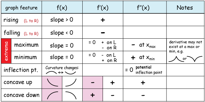
Figure 10
Example 3
Sketch an accurate graph of f(x) including the locations of any asymptotes, maxima, minima and inflection points.
[latex]{f(x)}=\frac{{{x}^{2}-{2x}+{4}}}{{{x}-{2}}}[/latex]
First, we note the the numerator is quadratic, with a negative discriminant, therefore the function has no real roots and its graph doesn't cross the x-axis:
[latex]{b}^{2}-{4ac}={-2}^{2}-{4(1)(-2)}={4}-{8}={-4}[/latex]
The degree of the numerator (2) exceeds the degree of the denominator (1) by one, so the function has a slant asymptote. We find its equation by polynomial division, then note that the denominator has a zero at x = 2, therefore the function has a vertical asymptote there.

Now we find the extrema by taking the first derivative of f(x), then setting it equal to zero and solving for x.

Two zeros result, one at x = 0 and the other at x = 4. Now we take the derivative of the derivative, f″(x), to look for inflection points (f″(x) = 0), and to test whether our extrema are minima or maxima. This time I won't take up the space to calculate the second derivative of f(x), I'll just give the answer. You, however, should confirm that the answer is correct!

Looking back at our table of reminders, we see that if the second derivative is negative at an extreme value of the function domain, then there's a relative maximum there, and the opposite is true for a minimum. Notice that both the value of f′(x) and f″(x) are undefined at x = 2, as we would expect if there is a vertical asymptote at x = 2.

Figure 11
Example 4
Sketch an accurate graph of f(x) including the locations of any asymptotes, maxima, minima and inflection points.

The numerator is factorable, with real roots at x = 3 and x = −2, so we know that the graph crosses the x-axis at those (and only those) points. We can also easily see that the denominator is zero for x = 1, so there's a vertical asymptote at x = 1. There are no holes in the graph because there are no binomials (a + b) common to both the numerator and denominator.
It's also easy at this point to notice that the function crosses the y-axis at f(0) = 6:

The y-intercept is often very easy to calculate, so don't ignore it. Now we note the the degree of the denominator is one less than that of the numerator, so we expect a slanted asymptote, and we find its equation by polynomial division:

Now to find any maxima or minima, if they exist, we find the first derivative, f′(x), and set it equal to zero:
 Setting the derivative equal to zero (below) , and solving by completing the square shows us that there are no real solutions, thus there are no places on the curve with a horizontal tangent slope—no maxima or minima at all:
 Here is the graph of f(x).

Figure 12
Example 5
Sketch the graph of the function f(x) = x3 − 2x2 − 5x + 6
First, try to factor such a function; it could make life easier. This function can't be factored by grouping, but the rational root theorem, with a guess of x = 1 gets us to a factorable quadratic:

So we know that the graph crosses the x-axis at x = 1, −2 and 3. That's useful information.
Now the first derivative of f(x) is f′(x) = 3x2 − 4x − 5. Setting this to zero and finding the roots by completing the square (don't forget that!) gives two real roots:

So there is one maximum and one minimum (think about it, there can't be two maxima or two minima without the opposite intervening), but we don't know which is which. We can figure it out in two ways.
First, if the derivative is increasing on the left side of an extremum and decreasing on the right, the extremum is a maximum. The square root of 19 is about 4.5, so our extrema lie at about x = +2 and x = −2/3. Now f′(−1) is positive and f′(0) is negative, so the leftmost extremum is a maximum. Then f′(1) is negative and f′(3) is positive, so the other extremum is a minimum.
Second, we can apply the second derivative test. We have:
 The two methods are in agreement.

Figure 13
Example 6
Explore the graph of the absolute-value function
 .
.
Absolute value functions are tricky because they always have sharp points, like at the bottom of the V-shaped graph of y = |x|. These are called cusps. A cusp is a point in a graph where two branches meet, but the tangents of each branch are not equal.
In order to analyze this graph, we'll have to take the derivative of an absolute-value function, and that's a little tricky. To do it, we need to define the absolute value of a number as the square root of the square of that number. That makes sense: If we square a negative number, the result is positive, then we recover the number (without the negative sign) by taking the square root. The definition is in the box below.

Solution
According to the differentiation formula, f′(x) is:

Then if we set the derivative equal to zero, we get three solutions

Two of the solutions, x = ±1 are cusps. While the function is continuous at these points (you wouldn't have to lift your pencil to trace it), it is not differentiable.

Figure 14
Example 7
Sketch the graph of the function f(x) = 3x1/3
We know the general shape of a root function, but recall that we can find odd roots of negative numbers, so this function is somewhat S-shaped.
Take the first derivative and notice that it is greater than zero for all x, and x can't be equal to zero. So this function is increasing throughout its domain, which includes zero, but its slope is undefined at zero.

The second derivative shows us that the function is concave-upward for x < 0 and concave downward for x > 0. The second derivative, too, is undefined at x = 0.

You can see the graph of the function in figure 15. It is continuous over its domain, (−∞, ∞), but non-differentiable at x = 0.

Figure 15
Licenses & Attributions
CC licensed content, Shared previously
