Vector Functions
Vector-Valued Functions
A vector function covers a set of multidimensional vectors at the intersection of the domains of [latex]f[/latex], [latex]g[/latex], and [latex]h[/latex].Learning Objectives
Describe application of the vector valued functionsKey Takeaways
Key Points
- A vector valued function can be made up of vectors and/or scalars.
- Each component function in a vector valued function represents the location of the value in a different dimension.
- The domain of the vector value function is the intersection of the component function domains.
- Vector valued functions can behave the same ways as vectors, and be evaluated similarly.
Key Terms
- domain: the set of all possible mathematical entities (points) where a given function is defined
- vector: a directed quantity, one with both magnitude and direction; the signed difference between two points
- scalar: a quantity that has magnitude but not direction; compare vector
What is a Vector Valued Function?
Also called vector functions, vector valued functions allow you to express the position of a point in multiple dimensions within a single function. These can be expressed in an infinite number of dimensions, but are most often expressed in two or three. The input into a vector valued function can be a vector or a scalar. In this atom we are going to introduce the properties and uses of the vector valued functions.Properties of Vector Valued Functions
A vector valued function allows you to represent the position of a particle in one or more dimensions. A three-dimensional vector valued function requires three functions, one for each dimension. In Cartesian form with standard unit vectors (i,j,k), a vector valued function can be represented in either of the following ways: [latex]\mathbf{r}(t) = f(t)\mathbf{i} + g(t)\mathbf{j} + h(t)\mathbf{k}\\ \mathbf{r}(t) = \langle f(t), g(t), h(t) \rangle[/latex] where [latex]t[/latex] is being used as the variable. This is a three dimensional vector valued function. The graph shows a visual representation of [latex]\mathbf{r}(t) = \langle 2 \cos(t), 4 \sin(t), t \rangle[/latex].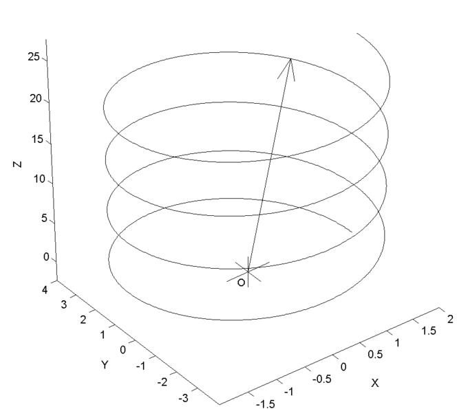
Vector-Valued Function: This a graph of a parametric curve (a simple vector-valued function with a single parameter of dimension [latex]1[/latex]). The graph is of the curve: [latex]\langle 2 \cos(t), 4 \sin(t),t \rangle[/latex] where [latex]t[/latex] goes from [latex]0[/latex] to [latex]8 \pi[/latex].
Example
For this example, we will use time as our parameter. The following vector valued function represents time, [latex]t[/latex]: [latex-display]\mathbf{r}(t) = f(t)\mathbf{i} + g(t)\mathbf{j} + h(t)\mathbf{k}[/latex-display] This function is representing a position. Therefore, if we take the derivative of this function, we will get the velocity: [latex-display]\displaystyle{\frac{d\mathbf{r}(t)}{dt}= f(t)\mathbf{i}' + g(t)\mathbf{j}' + h(t)\mathbf{k}' \\ \,\qquad = \mathbf{v}(t)\\ }[/latex-display] If we differentiate a second time, we will be left with acceleration: [latex-display]\displaystyle{\frac{d\mathbf{v}(t)}{dt}= \mathbf{a}(t)}[/latex-display]Arc Length and Speed
Arc length and speed are, respectively, a function of position and its derivative with respect to time.Learning Objectives
Distinguish the arc length and speedKey Takeaways
Key Points
- Arc length is found by placing a number of points along a curve, connecting them by line segments, and then adding those segment lengths together.
- The beginning of deriving the formula for arc length starts with Pythagoras's theorem.
- When finding the arc length, the integral used needs to be with respect to position, [latex]x[/latex].
- When finding the speed along a curve, the integral used needs to be with respect to time, [latex]t[/latex].
Key Terms
- derivative: a measure of how a function changes as its input changes
- velocity: a vector quantity that denotes the rate of change of position with respect to time, or a speed with the directional component
Arc Length and Speed
Since length is a magnitude that involves position, it is easy to deduce that the derivative of a length, or position, will give you the velocity —also known as speed—of a function. This is because a derivative gives you a rate of change with respect to a parameter. Velocity is the rate of change of a position with respect to time. Let's start this atom by looking at arc length with calculus.Arc Length
The arc length is the length you would get if you took a curve, straightened it out, and then measured the length of that line. The arc length can be found using geometry, but for the sake of this atom, we are going to use integration. The arc length is approximated by connecting a finite number of points along and curve, connecting those lines to create a a string of very small straight lines, and adding them together. To find this using integration, we should start out by using the Pythagorean Theorem for length of the different sides of a triangle: [latex]\displaystyle{ds^2=dx^2+dy^2 \frac{ds^2}{dx^2}\\ \, \quad= 1+\frac{dy^2}{dx^2}ds \\ \, \quad=\sqrt{1+{\frac{dy^2}{dx^2}^2}} \cdot dx\\ \, \quad=\int^b_a\sqrt{1+f'(x)^2} \cdot dx}[/latex] where [latex]s[/latex] is the arc length. If [latex]x=X(t)[/latex] and [latex]y=Y(t)[/latex], [latex]\displaystyle{s =\int^b_a\sqrt{1+{f'(x)}^2} \cdots dx\\ \,\,=\int^b_a\sqrt{[X'(t)]^2+[Y'(t)] \cdots dt}\\ \,\,= \int^b_a\sqrt{dx^2+dy^2}\\ \,\,= \int^b_a\sqrt{\frac{dx}{dt}^2+\frac{dy}{dt}^2 \cdots dt}}[/latex] Since this is a function of position and is defined by x, we need to have a derivative that is in respect to x: [latex-display]\int^b_a\sqrt{1+\frac{dy}{dx}^2*dx}[/latex-display]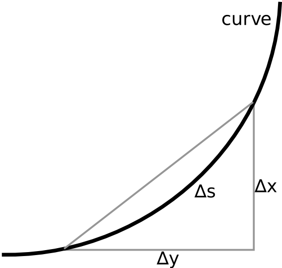
Curves and the Pythagorean Theorem: For a small piece of curve, ∆s can be approximated with the Pythagorean theorem.
Arc Length: The arc length is the equivalent of taking a curve, straightening it out, and then measuring it, as seen in this animation.
Arc Speed
Now that the hard part is over, we can easily find the speed along this curve. Since speed is in relation to time and not position, we need to revert back to the arc length with respect to time: [latex-display]\displaystyle{\int^b_a\sqrt{\frac{dx}{dt}^2+\frac{dy}{dt}^2\cdot dt}}[/latex-display] Then, differentiate with respect to time: [latex-display]\displaystyle{v(t)=s'=\sqrt{[X'(t)]^2+[Y'(t)]^2}}[/latex-display]Calculus of Vector-Valued Functions
A vector function is a function that can behave as a group of individual vectors and can perform differential and integral operations.Learning Objectives
Discuss how vector functions are manipulatedKey Takeaways
Key Points
- A vector valued function can be made up of vectors and/or scalars.
- Each component function in a vector valued function represents the location of the value in a different dimension.
- Vector valued functions can behave the same ways as vectors, and be evaluated similarly.
- Vector functions are widely used in the study of electromagnetic fields, gravitation fields, and fluid flow.
Key Terms
- vector: a directed quantity, one with both magnitude and direction; the signed difference between two points
- scalar: a quantity that has magnitude but not direction; compare vector
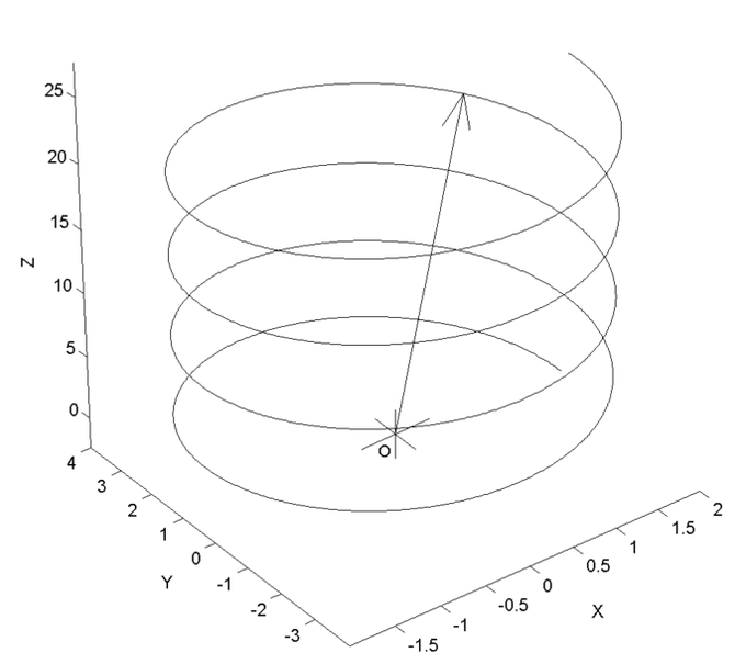
Vector valued function: This graph is a visual representation of the three-dimensional vector-valued function [latex]\mathbf{r}(t) = \langle 2 \cos(t), 4 \sin(t), t \rangle[/latex]. This can be broken down into three separate functions called component functions: [latex]x(t) = 2 \cos(t)y(t) = 4 \sin(t)z(t) = t[/latex].
Arc Length and Curvature
The curvature of an object is the degree to which it deviates from being flat and can be found using arc length.Learning Objectives
Explain the relationship between the curvature of an object and the arc lengthKey Takeaways
Key Points
- The arc length is a function of position, so its derivative will be a function of time. This can give you the rate of change of the position, in relation to time, which is called the curvature.
- The curvature can be found by taking the derivative of the velocity vector, which is given: [latex]\Vert\frac{dT}{ds}\Vert[/latex].
- This same magnitude can also be found using the concept of calculus, the limit.
Key Terms
- sharpness: the fineness of the point a pointed object
- curvature: the degree to which an objet deviates from being flat
- normal: a line or vector that is perpendicular to another line, surface, or plane
Arc Curvature
The curvature of an arc is a value that represents the direction and sharpness of a curve. On any curve, there is a center of curvature, C. This is the intersection point of two infinitely close normals to this curve. The radius, R, is the distance from this intersection point to the center of curvature.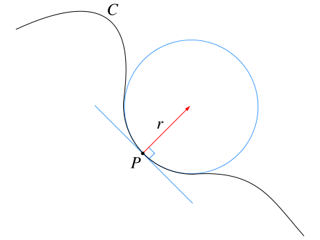
Curvature: Curvature is the amount an object deviates from being flat. Given any curve C and a point P on it, there is a unique circle or line which most closely approximates the curve near P\. The curvature of C at P is then defined to be the curvature of that circle or line. The radius of curvature is defined as the reciprocal of the curvature.
How Does This Relate to Arc Length?
The curvature can also be approximated using limits. Given the points P and Q on the curve, lets call the arc length s(P,Q), and the linear distance from P to Q will be denoted as d(P,Q). The curvature of the arc at point P can be found by obtaining the limit: [latex-display]\kappa(P) = \frac{\lim}{Q\rightarrow P}\sqrt{\frac{24*(s(P,Q)-d(P,Q))}{s(P,Q)^3}}[/latex-display] In order to use this formula, you must first obtain the arc length of the curve from points P to Q and length of the linear segment that connect points P and Q. In a previous atom, we went into more detail on how to find the arc length, but for the sake of this atom we will just restate those formulas:In Cartesian coordinates: [latex-display]\int^b_a\sqrt{1+\frac{dy}{dx}^2*dx}\\ [/latex-display]Planetary Motion According to Kepler and Newton
Kepler explained that the planets move in an ellipse around the Sun, which is at one of the two foci of the ellipse.Learning Objectives
Identify three laws of planetary motion formulated by Johannes KeplerKey Takeaways
Key Points
- Kepler's first law of planetary motion describes the motion of its orbit around the Sun.
- Kepler's second law of planetary motion explains the reason why the planet moves faster as it approaches the Sun, and slower as it moves farther away.
- Kepler's third law of planetary motion explains how the period of an orbit is related to the semi-major axis of its orbit.
- Newton takes the information presented by Kepler and uses it to explain that the value of a force on an object is the product of its mass and its orbital acceleration.
- Newton also clarifies that the orbit is an elliptical shape because while each planet is attracted to the Sun, they are also attracted to each other.
Key Terms
- gravitational constant: an empirical physical constant involved in the calculation of the gravitational attraction between objects with mass
- eccentricity: the ratio—constant for any particular conic section—of the distance of a point from the focus to its distance from the directrix
- ellipse: a closed curve; the locus of a point such that the sum of the distances from that point to two other fixed points (called the foci of the ellipse) is constant; equivalently, the conic section that is the intersection of a cone with a plane that does not intersect the base of the cone
Kepler's First Law
As we already stated, the first law of planetary motion states that the orbit of every planet is an ellipse with the Sun at one focus. In order to discuss this law, and the laws that follow, we should examine the components of an ellipse a bit more closely. The eccentricity of an ellipse tells you how stretched out the ellipse is. The eccentricity can be from 0 to 1. If the eccentricity is equal to zero, that means it is a circle. In Kepler's time, the extremes of planetary eccentricity were Venus, 0.007, and Mercury, 0.2. The eccentricity is what makes an ellipse different from a circle. [latex-display]\displaystyle{r=\frac{p}{1+{\Sigma} \cdot \cos{\theta}}}[/latex-display] where [latex]p[/latex] is the semi-latus rectum, [latex]\Sigma[/latex] is the eccentricity, [latex]r[/latex] is the distance between the planet and the sun, and [latex]\theta[/latex] is the angle between the position of the planet and its most direct route to the Sun. The minimum distance occurs when the angle is 0. The maximum distance occurs when the angle is 180 degrees. These values are important because the equation for eccentricity is: [latex-display]\displaystyle{\Sigma=\frac{r_{\text{max}}-r_{\text{min}}}{r_{\text{max}}+r_{\text{min}}}}[/latex-display] The semi-major axis, [latex]a[/latex], can be found as follows: [latex-display]\displaystyle{a=\frac{p}{1-\Sigma^2}}[/latex-display] The semi-minor axis, [latex]b[/latex], can be found as follows: [latex-display]\displaystyle{b=\frac{p}{\sqrt{1-\Sigma^2}}}[/latex-display] The area of an ellipse is found as follows: [latex-display]A=\pi \cdot a \cdot b[/latex-display]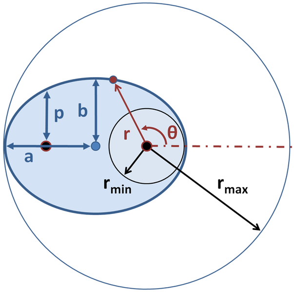
Ellipse: The important components of an ellipse are as follows: semi-major axis [latex]a[/latex], semi-minor axis [latex]b[/latex], semi-latus rectum [latex]p[/latex], the center of the ellipse, and its two foci marked by large dots. For [latex]\theta = 0[/latex] degrees, [latex]r = r_{\text{min}}[/latex] and for [latex]\theta = 180[/latex] degrees, [latex]r = r_{\text{max}}[/latex].
Kepler's Second Law
The second law of planetary motion states that in an amount of time, [latex]t[/latex], a line from the planet to the Sun will sweep out a triangle having a base of [latex]r[/latex] and a height of [latex]r \cdot d\theta[/latex]. Therefore, the area of this triangle is: [latex-display]\displaystyle{dA=\frac{1}{2} \cdot r \cdot rd\theta}[/latex-display] and the ratio of the area of this triangle to the time elapsed is: [latex-display]\displaystyle{\frac{dA}{dt}=\frac{1}{2} \cdot r^2 \cdot \frac{d\theta}{dt}}[/latex-display] As the planet moves closer to the Sun, it speeds up. This allows the triangle to have an equal area in an equal amount of time regardless of position of the planet. As we learned in the first section, the area of an ellipse is [latex]\pi \cdot a \cdot b[/latex]. Therefore, the period ([latex]P[/latex]) of the ellipse satisfies: [latex]\pi \cdot a \cdot b=P \cdot \frac{1}{2} \cdot r^2 \cdot \theta\\ r^2\theta=n\cdot a\cdot b[/latex] where [latex]\theta[/latex] is the angular velocity with respect to time, and [latex]n[/latex] is the mean motion of the planet around the Sun.
The Second Law: Illustration of Kepler's second law. The planet moves faster near the Sun so that the same area is swept out in a given time as it would be at larger distances, where the planet moves more slowly. The green arrow represents the planet's velocity, and the purple arrows represent the force on the planet.
Kepler's Third Law
Kepler's third law describes the relationship between the distance of the planets from the Sun, and their orbits period. [latex]P^2 \propto a^3[/latex], with a constant of proportionality of: [latex-display]\displaystyle{\frac{P^2_{\text{planet}}}{a^3_{\text{planet}}} = \frac{P^2_{\text{earth}}}{a^3_{\text{earth}}} = 1 \frac{\text{year}}{\text{AU}}}[/latex-display] where AU is an astronomical unit. In the case of a circular orbit, the proportionality constant is as follows: [latex-display]\displaystyle{\frac{4\pi^2}{T^2}=\frac{GM}{R^3}}[/latex-display] where [latex]T[/latex] is the period, [latex]G[/latex] is the gravitational constant, and [latex]R[/latex] is the distance between the center of mass of the two bodies.How does Newton Relate to Kepler?
Newton derived his theory of the acceleration of a planet from Kepler's first and second laws. Newton theorized that the direction of a planet is always towards the Sun. In addition, the magnitude of the acceleration is inversely proportional to the square of its distance from the Sun. From this, Newton defined the force acting on a planet as the product of its mass and acceleration. Therefore, by Newton's law, every planet is attracted to the Sun, and the force acting on a planet is directly proportional to the mass and inversely proportional to the square of its distance from the Sun.Tangent Vectors and Normal Vectors
A vector is normal to another vector if the intersection of the two form a 90-degree angle at the tangent point.Learning Objectives
Distinguish tangent vectors and normal vectorsKey Takeaways
Key Points
- In order for one vector to be tangent to another vector, the intersection needs to be exactly 90 degrees. On a curve or an uneven object, each point will have a unique normal vector.
- If you want to check whether two vectors are normal to each other, you can find the dot product of the two and make sure it equals zero.
- If you want to find out exactly what the angle between the two vectors is, you can use the following equation, which also employs the dot product: [latex]\mathbf{a} \bullet \mathbf{b} = \left|\mathbf{a}\right| \left|\mathbf{b}\right| \cos \theta[/latex].
- In order to find the tangent vector to another vector or object, just take the derivative of the reference vector.
Key Terms
- tangent: a straight line touching a curve at a single point without crossing it there
- perpendicular: at or forming a right angle (to)
Normal Vectors
An object is normal to another object if it is perpendicular to the point of reference. That means that the intersection of the two objects forms a right angle. Usually, these vectors are denoted as [latex]\mathbf{n}[/latex].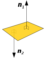
Figure 1: Normal Vector: These vectors are normal to the plane because the intersection between them and the plane makes a right angle.
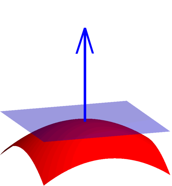
Figure 2: Normal Plane: A plane can be determined as normal to the object if the directional vector of the plane makes a right angle with the object at its tangent point. This plane is normal to the point on the sphere to which it is tangent. Each point on the sphere will have a unique normal plane.
Dot Product
As we covered in another atom, one of the manipulations of vectors is called the Dot Product. When you take the dot product of two vectors, your answer is in the form of a single value, not a vector. In order for two vectors to be normal to each other, the dot product has to be zero. [latex]\mathbf{a} \bullet \mathbf{b} = 0\\ \,\,\,\quad = a_1b_1+a_2b_2+a_3b_3\\ \,\,\,\quad = \left|\mathbf{a}\right| \left|\mathbf{b}\right| \cos \theta[/latex]Tangent Vectors
Tangent vectors are almost exactly like normal vectors, except they are tangent instead of normal to the other vector or object. These vectors can be found by obtaining the derivative of the reference vector, [latex]\mathbf{r}(t)[/latex]: [latex-display]\mathbf{r}(t) = f(t)\mathbf{i}+g(t)\mathbf{j}+h(t)\mathbf{k}[/latex-display]Licenses & Attributions
CC licensed content, Shared previously
- Curation and Revision. Provided by: Boundless.com License: CC BY-SA: Attribution-ShareAlike.
CC licensed content, Specific attribution
- Vector-valued function. Provided by: Wikipedia License: CC BY-SA: Attribution-ShareAlike.
- scalar. Provided by: Wiktionary License: CC BY-SA: Attribution-ShareAlike.
- domain. Provided by: Wiktionary License: CC BY-SA: Attribution-ShareAlike.
- vector. Provided by: Wiktionary License: CC BY-SA: Attribution-ShareAlike.
- Vector-Valued Function. Provided by: WikiPedia License: Public Domain: No Known Copyright.
- Arc length. Provided by: Wikipedia License: CC BY-SA: Attribution-ShareAlike.
- derivative. Provided by: Wikipedia License: CC BY-SA: Attribution-ShareAlike.
- velocity. Provided by: Wiktionary License: CC BY-SA: Attribution-ShareAlike.
- Vector-Valued Function. Provided by: WikiPedia License: Public Domain: No Known Copyright.
- Arc length. Provided by: Wikipedia License: Public Domain: No Known Copyright.
- Arclength-approx. Provided by: Wikipedia License: CC BY-SA: Attribution-ShareAlike.
- Vector calculus. Provided by: Wikipedia License: CC BY-SA: Attribution-ShareAlike.
- Vector-valued function. Provided by: Wikipedia License: CC BY-SA: Attribution-ShareAlike.
- scalar. Provided by: Wiktionary License: CC BY-SA: Attribution-ShareAlike.
- vector. Provided by: Wiktionary License: CC BY-SA: Attribution-ShareAlike.
- Vector-Valued Function. Provided by: WikiPedia License: Public Domain: No Known Copyright.
- Arc length. Provided by: Wikipedia License: Public Domain: No Known Copyright.
- Arclength-approx. Provided by: Wikipedia License: CC BY-SA: Attribution-ShareAlike.
- Wikipedia. Provided by: Wikipedia License: CC BY-SA: Attribution-ShareAlike.
- Curvature. Provided by: Wikipedia License: CC BY-SA: Attribution-ShareAlike.
- normal. Provided by: Wiktionary License: CC BY-SA: Attribution-ShareAlike.
- sharpness. Provided by: Wiktionary License: CC BY-SA: Attribution-ShareAlike.
- curvature. Provided by: Wiktionary License: CC BY-SA: Attribution-ShareAlike.
- Vector-Valued Function. Provided by: WikiPedia License: Public Domain: No Known Copyright.
- Arc length. Provided by: Wikipedia License: Public Domain: No Known Copyright.
- Arclength-approx. Provided by: Wikipedia License: CC BY-SA: Attribution-ShareAlike.
- Wikipedia. Provided by: Wikipedia License: CC BY-SA: Attribution-ShareAlike.
- Osculating circle. Provided by: Wikipedia License: Public Domain: No Known Copyright.
- Kepler's laws of planetary motion. Provided by: Wikipedia License: CC BY-SA: Attribution-ShareAlike.
- Boundless. Provided by: Boundless Learning License: CC BY-SA: Attribution-ShareAlike.
- ellipse. Provided by: Wiktionary Located at: https://en.wiktionary.org/wiki/ellipse. License: CC BY-SA: Attribution-ShareAlike.
- gravitational constant. Provided by: Wiktionary License: CC BY-SA: Attribution-ShareAlike.
- Vector-Valued Function. Provided by: WikiPedia License: Public Domain: No Known Copyright.
- Arc length. Provided by: Wikipedia License: Public Domain: No Known Copyright.
- Arclength-approx. Provided by: Wikipedia License: CC BY-SA: Attribution-ShareAlike.
- Wikipedia. Provided by: Wikipedia License: CC BY-SA: Attribution-ShareAlike.
- Osculating circle. Provided by: Wikipedia License: Public Domain: No Known Copyright.
- Kepler-second-law. Provided by: Wikipedia License: CC BY-SA: Attribution-ShareAlike.
- Ellipse latus rectum. Provided by: Wikipedia License: CC BY: Attribution.
- Normal vector. Provided by: Wikipedia License: CC BY-SA: Attribution-ShareAlike.
- tangent. Provided by: Wiktionary License: CC BY-SA: Attribution-ShareAlike.
- perpendicular. Provided by: Wikipedia License: CC BY-SA: Attribution-ShareAlike.
- Vector-Valued Function. Provided by: WikiPedia License: Public Domain: No Known Copyright.
- Arc length. Provided by: Wikipedia License: Public Domain: No Known Copyright.
- Arclength-approx. Provided by: Wikipedia License: CC BY-SA: Attribution-ShareAlike.
- Wikipedia. Provided by: Wikipedia License: CC BY-SA: Attribution-ShareAlike.
- Osculating circle. Provided by: Wikipedia License: Public Domain: No Known Copyright.
- Kepler-second-law. Provided by: Wikipedia License: CC BY-SA: Attribution-ShareAlike.
- Ellipse latus rectum. Provided by: Wikipedia License: CC BY: Attribution.
- Normal vectors2. Provided by: Wikipedia License: Public Domain: No Known Copyright.
- Surface normal illustration. Provided by: Wikipedia License: Public Domain: No Known Copyright.
