Vector Calculus
Vector Fields
A vector field is an assignment of a vector to each point in a subset of Euclidean space.Learning Objectives
Describe construction of vector fieldsKey Takeaways
Key Points
- A vector field in the plane, for instance, can be visualized as a collection of arrows with a given magnitude and direction each attached to a point in the plane.
- Vector fields can be constructed out of scalar fields using the gradient operator.
- Vector fields can be thought to represent the velocity of a moving flow in space, and this physical intuition leads to notions such as the divergence (the rate of change of volume of a flow) and curl (the rotation of a flow).
Key Terms
- vector field: a construction in which each point in a Euclidean space is associated with a vector; a function whose range is a vector space
- bijective: both injective and surjective

Fig 1
Examples
- A vector field for the movement of air on Earth will associate for every point on the surface of the Earth a vector with the wind speed and direction for that point.
- A gravitational field generated by any massive object is a vector field. For example, the gravitational field vectors for a spherically symmetric body would all point towards the sphere's center, with the magnitude of the vectors reducing as radial distance from the body increases.
- Magnetic field lines can be revealed using small iron filings.
- In the case of the velocity field of a moving fluid, a velocity vector is associated to each point in the fluid.
Conservative Vector Fields
A conservative vector field is a vector field which is the gradient of a function, known in this context as a scalar potential.Learning Objectives
Identify properties of conservative vector fieldsKey Takeaways
Key Points
- Conservative vector fields have the following property: The line integral from one point to another is independent of the choice of path connecting the two points; it is path-independent.
- Conservative vector fields are also irrotational, meaning that (in three dimensions) they have vanishing curl.
- A vector field [latex]\mathbf{v}[/latex] is said to be conservative if there exists a scalar field [latex]\varphi[/latex] such that [latex]\mathbf{v}=\nabla\varphi[/latex].
Key Terms
- vector field: a construction in which each point in a Euclidean space is associated with a vector; a function whose range is a vector space
- bijective: both injective and surjective

Fig 1: The above field [latex]\mathbf{v}(x,y,z) = (\frac{−y}{x^2+y^2}, \frac{x}{x^2+y^2}, 0)[/latex] includes a vortex at its center, meaning it is non-irrotational; it is neither conservative, nor does it have path independence. However, any simply connected subset that excludes the vortex line [latex](0,0,z)[/latex] will have zero curl, [latex]\nabla \mathbf{v}=0[/latex]. Such vortex-free regions are examples of irrotational vector fields.
Path Independence
A key property of a conservative vector field is that its integral along a path depends only on the endpoints of that path, not the particular route taken. Suppose that [latex]S\subseteq\mathbb{R}^3[/latex]is a region of three-dimensional space, and that [latex]P[/latex] is a rectifiable path in [latex]S[/latex] with start point [latex]A[/latex] and end point [latex]B[/latex]. If [latex]\mathbf{v}=\nabla\varphi[/latex] is a conservative vector field, then the gradient theorem states that [latex]\int_P \mathbf{v}\cdot d\mathbf{r}=\varphi(B)-\varphi(A)[/latex]. This holds as a consequence of the Chain Rule and the Fundamental Theorem of Calculus. An equivalent formulation of this is to say that [latex]\oint \mathbf{v}\cdot d\mathbf{r}=0[/latex] for every closed loop in [latex]S[/latex].
Line Integral Over Scalar Field: The line integral over a scalar field [latex]f[/latex] can be thought of as the area under the curve [latex]C[/latex] along a surface [latex]z=f(x,y)[/latex], described by the field.
Line Integrals
A line integral is an integral where the function to be integrated is evaluated along a curve.Learning Objectives
Calculate the value of a line integralKey Takeaways
Key Points
- The value of the line integral is the sum of the values of the field at all points on the curve, weighted by some scalar function on the curve (commonly arc length or, for a vector field, the scalar product of the vector field with a differential vector in the curve).
- Many simple formulae in physics (for example, [latex]W=F·s[/latex]) have natural continuous analogs in terms of line integrals ([latex]W= \int_C F\cdot ds[/latex]). The line integral finds the work done on an object moving through an electric or gravitational field, for example.
- In qualitative terms, a line integral in vector calculus can be thought of as a measure of the total effect of a given field along a given curve.
Key Terms
- vector field: a construction in which each point in a Euclidean space is associated with a vector; a function whose range is a vector space
- bijective: both injective and surjective
Line Integral Over Scalar Field: The line integral over a scalar field [latex]f[/latex] can be thought of as the area under the curve [latex]C[/latex] along a surface [latex]z = f(x,y)[/latex], described by the field.
Line Integral of a Scalar Field
For some scalar field [latex]f:U \subseteq R^n \to R[/latex], the line integral along a piecewise smooth curve [latex]C \subset U[/latex] is defined as: [latex-display]\int_C f\, ds = \int_a^b f(\mathbf{r}(t)) |\mathbf{r}'(t)|\, dt[/latex-display] where [latex]r: [a, b] \to C[/latex] is an arbitrary bijective parametrization of the curve [latex]C[/latex] such that [latex]r(a)[/latex] and [latex]r(b)[/latex] give the endpoints of [latex]C[/latex] and [latex]a[/latex].Line Integral of a Vector Field
For a vector field [latex]\mathbf{F}: U \subseteq R^n \to R^n[/latex], the line integral along a piecewise smooth curve [latex]C \subset U[/latex], in the direction of [latex]r[/latex], is defined as: [latex-display]\displaystyle{\int_C \mathbf{F}(\mathbf{r})\cdot\,d\mathbf{r} = \int_a^b \mathbf{F}(\mathbf{r}(t))\cdot\mathbf{r}'(t)\,dt}[/latex-display] where [latex]\cdot[/latex] is the dot product and [latex]r: [a, b] \to C[/latex] is a bijective parametrization of the curve [latex]C[/latex] such that [latex]r(a)[/latex] and [latex]r(b)[/latex] give the endpoints of [latex]C[/latex].Fundamental Theorem for Line Integrals
Gradient theorem says that a line integral through a gradient field can be evaluated from the field values at the endpoints of the curve.Learning Objectives
Discuss application of the gradient theorem in physicsKey Takeaways
Key Points
- The gradient theorem implies that line integrals through irrotational vector fields are path-independent.
- Work done by conservative forces, described by a vector field, does not depend on the path followed by the object, but only the end points, as the above equation shows.
- Any conservative vector field can be expressed as the gradient of a scalar field.
Key Terms
- differentiable: having a derivative, said of a function whose domain and co-domain are manifolds
- vector field: a construction in which each point in a Euclidean space is associated with a vector; a function whose range is a vector space
- conservative force: a force with the property that the work done in moving a particle between two points is independent of the path taken

Electric Field Lines of a Positive Charge: Electric field lines emanating from a point where positive electric charge is suspended over a negatively charged infinite sheet. Electric field is a vector field which can be represented as a gradient of a scalar field, called electric potential. Therefore, electric force is a conservative force.
Proof
If [latex]\varphi[/latex] is a differentiable function from some open subset [latex]U[/latex] (of [latex]R^n[/latex]) to [latex]R[/latex], and if [latex]r[/latex] is a differentiable function from some closed interval [latex][a,b][/latex] to [latex]U[/latex], then by the multivariate chain rule, the composite function [latex]\circ r[/latex] is differentiable on [latex](a,b)[/latex] and [latex]\frac{d}{dt}(\varphi \circ \mathbf{r})(t)=\nabla \varphi(\mathbf{r}(t)) \cdot \mathbf{r}'(t)[/latex] for for all [latex]t[/latex] in [latex](a,b)[/latex]. Here the [latex]\cdot[/latex] denotes the usual inner product. Now suppose the domain [latex]U[/latex] of [latex]\varphi[/latex] contains the differentiable curve [latex]\gamma[/latex] with endpoints [latex]p[/latex] and [latex]q[/latex] (oriented in the direction from [latex]p[/latex] to [latex]q[/latex]). If [latex]r[/latex] parametrizes for [latex]t[/latex] in [latex][a,b][/latex], then the above shows that [latex]\begin{align} \int_{\gamma} \nabla\varphi(\mathbf{u}) \cdot d\mathbf{u} &=\int_a^b \nabla\varphi(\mathbf{r}(t)) \cdot \mathbf{r}'(t)dt \\ &=\int_a^b \frac{d}{dt}\varphi(\mathbf{r}(t))dt \\ &=\varphi(\mathbf{r}(b))-\varphi(\mathbf{r}(a))\\ &=\varphi\left(\mathbf{q}\right)-\varphi\left(\mathbf{p}\right) \end{align}[/latex] where the definition of the line integral is used in the first equality and the fundamental theorem of calculus is used in the third equality.Green's Theorem
Green's theorem gives relationship between a line integral around closed curve [latex]C[/latex] and a double integral over plane region [latex]D[/latex] bounded by [latex]C[/latex].Learning Objectives
Explain the relationship between the Green's theorem, the Kelvin–Stokes theorem, and the divergence theoremKey Takeaways
Key Points
- Green's theorem is a special case of the Kelvin–Stokes theorem, when applied to a region in the [latex]xy[/latex]-plane.
- Considering only two-dimensional vector fields, Green's theorem is equivalent to the two-dimensional version of the divergence theorem.
- Green's theorem can be used to compute area by line integral.
Key Terms
- double integral: An integral extended to functions of more than one real variable
- line integral: An integral the domain of whose integrand is a curve.

Computing area by line integral: [latex]D[/latex] is a simple region with its boundary consisting of the curves [latex]C_1[/latex], [latex]C_2[/latex], [latex]C_3[/latex], [latex]C_4[/latex]. Green's theorem can be used to compute area by line integral. The area is given by [latex]A = \iint_{D}\mathrm{d}A[/latex]. Provided we choose [latex]L[/latex] and [latex]M[/latex] such that: [latex]\frac{\partial M}{\partial x} - \frac{\partial L}{\partial y} = 1[/latex], then the area is given by [latex]A=\oint_{C} x[/latex]. Possible formulas for the area of [latex]D[/latex] include: [latex]A=\oint_{C} xdy[/latex], [latex]A = -\oint_{C} ydx[/latex], and [latex]A = \frac{1}{2}\oint_{C} (xdy - ydx)[/latex].
Curl and Divergence
The four most important differential operators are gradient, curl, divergence, and Laplacian.Learning Objectives
Calculate the direction and the magnitude of the curl, and the magnitude of the divergenceKey Takeaways
Key Points
- The curl is a vector operator that describes the infinitesimal rotation of a three-dimensional vector field.
- The direction of the curl is the axis of rotation, as determined by the right-hand rule, and the magnitude of the curl is the magnitude of rotation.
- Divergence is a vector operator that measures the magnitude of a vector field's source or sink at a given point in terms of a signed scalar.
Key Terms
- gradient: of a function [latex]y = f(x)[/latex] or the graph of such a function, the rate of change of [latex]y[/latex] with respect to [latex]x[/latex]; that is, the amount by which [latex]y[/latex] changes for a certain (often unit) change in [latex]x[/latex]
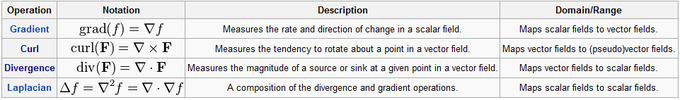
Four Most Important Differential Operators: Gradient, curl, divergence, and Laplacian are four most important differential operators.
Curl
The curl is a vector operator that describes the infinitesimal rotation of a 3-dimensional vector field. At every point in the field, the curl of that field is represented by a vector. The attributes of this vector—length and direction—characterize the rotation at that point. The direction of the curl is the axis of rotation, as determined by the right-hand rule, and the magnitude of the curl is the magnitude of rotation. If the vector field represents the flow velocity of a moving fluid, then the curl is the circulation density of the fluid. A vector field whose curl is zero is called irrotational. The curl is a form of differentiation for vector fields. The corresponding form of the fundamental theorem of calculus is Stokes' theorem, which relates the surface integral of the curl of a vector field to the line integral of the vector field around the boundary curve. The curl of a vector field [latex]\mathbf{F}[/latex], denoted by [latex]\nabla \times \mathbf{F}[/latex], is defined at a point in terms of its projection onto various lines through the point. If [latex]\hat{\mathbf{n}}[/latex] is any unit vector, the projection of the curl of [latex]\mathbf{F}[/latex] onto [latex]\hat{\mathbf{n}}[/latex] is defined to be the limiting value of a closed line integral in a plane orthogonal to [latex]\hat{\mathbf{n}}[/latex] as the path used in the integral becomes infinitesimally close to the point, divided by the area enclosed. Curl is defined by: [latex-display]\displaystyle{(\nabla \times \mathbf{F}) \cdot \mathbf{\hat{n}} \ \overset{\underset{\mathrm{def}}{}}{=} \lim_{A \to 0}\left( \frac{1}{|A|}\oint_{C} \mathbf{F} \cdot d\mathbf{r}\right)}[/latex-display]Divergence
Divergence is a vector operator that measures the magnitude of a vector field's source or sink at a given point in terms of a signed scalar. More technically, the divergence represents the volume density of the outward flux of a vector field from an infinitesimal volume around a given point. In physical terms, the divergence of a three-dimensional vector field is the extent to which the vector field flow behaves like a source or a sink at a given point. It is a local measure of its "outgoingness"—the extent to which there is more exiting an infinitesimal region of space than entering it. If the divergence is nonzero at some point, then there must be a source or sink at that position. (Note that we are imagining the vector field to be like the velocity vector field of a fluid (in motion) when we use the terms flow, sink, and so on.) More rigorously, the divergence of a vector field [latex]\mathbf{F}[/latex] at a point [latex]p[/latex] is defined as the limit of the net flow of [latex]\mathbf{F}[/latex] across the smooth boundary of a three-dimensional region [latex]V[/latex] divided by the volume of [latex]V[/latex] as [latex]V[/latex] shrinks to [latex]p[/latex]. Formally: [latex-display]\displaystyle{\nabla \cdot \mathbf{F}(p) = \lim_{V \rightarrow \{p\}} \iint_{S(V)} \frac{\mathbf{F}\cdot\mathbf{n}}{\left|V\right| } dS}[/latex-display] where [latex]\left|V\right|[/latex] is the volume of [latex]V[/latex], [latex]S(V)[/latex] is the boundary of [latex]V[/latex], and the integral is a surface integral with n being the outward unit normal to that surface.Parametric Surfaces and Surface Integrals
A parametric surface is a surface in the Euclidean space [latex]R^3[/latex] which is defined by a parametric equation.Learning Objectives
Define the surface integral and identify a parametric surfaceKey Takeaways
Key Points
- Parametric representation is the most general way to specify a surface. The curvature and arc length of curves on the surface can both be computed from a given parametrization.
- The same surface admits many different parametrizations.
- A surface integral is a definite integral taken over a surface. It can be thought of as the double integral analog of the line integral.
Key Terms
- electric potential: the potential energy per unit charge at a point in a static electric field; voltage
- gradient: of a function [latex]y = f(x)[/latex] or the graph of such a function, the rate of change of [latex]y[/latex] with respect to [latex]x[/latex]; that is, the amount by which [latex]y[/latex] changes for a certain (often unit) change in [latex]x[/latex]
- curl: the vector field denoting the rotationality of a given vector field
Parametric Surface
A parametric surface is a surface in the Euclidean space [latex]R^3[/latex] which is defined by a parametric equation with two parameters: [latex]\vec r: \Bbb{R}^2 \rightarrow \Bbb{R}^3[/latex]. Parametric representation is the most general way to specify a surface. Surfaces that occur in two of the main theorems of vector calculus, Stokes' theorem and the divergence theorem, are frequently given in a parametric form. The curvature and arc length of curves on the surface can both be computed from a given parametrization.Examples
- The simplest type of parametric surfaces is given by the graphs of functions of two variables: [latex]z=f(x,y)[/latex]; [latex]\vec{r}(x,y)=(x,y,f(x,y))[/latex].
- Using the spherical coordinates, the unit sphere can be parameterized by [latex]\vec r(\theta,\phi) = (\cos\theta \sin\phi, \sin\theta \sin \phi, \cos\phi), 0 \leq \theta < 2\pi, 0 \leq \phi \leq \pi[/latex].
- The straight circular cylinder of radius [latex]R[/latex] about the [latex]x[/latex]-axis has the following parametric representation: [latex]\vec{r}(x,\phi)=(x,R \cos \phi, r \sin \phi)[/latex].
Surface integral
A surface integral is a definite integral taken over a surface. It can be thought of as the double integral analog of the line integral. Given a surface, one may integrate over its scalar fields (that is, functions which return scalars as values), and vector fields (that is, functions which return vectors as values). Surface integrals have many applications in physics, particularly within the classical theory of electromagnetism. We will study surface integral of vector fields and related theorems in the following atoms.
Kelvin-Stokes' Theorem: An illustration of the Kelvin–Stokes theorem, with surface [latex]\Sigma[/latex], its boundary [latex]\partial[/latex], and the "normal" vector [latex]\mathbf{n}[/latex].
Surface Integrals of Vector Fields
The surface integral of vector fields can be defined component-wise according to the definition of the surface integral of a scalar field.Learning Objectives
Explain relationship between surface integral of vector fields and surface integral of a scalar fieldKey Takeaways
Key Points
- The flux is defined as the quantity of fluid flowing through [latex]S[/latex] in unit amount of time.
- To find the flux, we need to take the dot product of [latex]\mathbf{v}[/latex] with the unit surface normal to [latex]S[/latex] at each point, which will give us a scalar field, and integrate the obtained field.
- This is expressed as [latex]\int_S {\mathbf v}\cdot \,d{\mathbf {S}} = \int_S {\mathbf v}\cdot {\mathbf n}\,dS=\iint_T {\mathbf v}(\mathbf{x}(s, t))\cdot \left({\partial \mathbf{x} \over \partial s}\times {\partial \mathbf{x} \over \partial t}\right) ds\, dt[/latex].
Key Terms
- vector field: a construction in which each point in a Euclidean space is associated with a vector; a function whose range is a vector space
- parametrization: Is the process of deciding and defining the parameters necessary for a complete or relevant specification of a model or geometric object.
- flux: the rate of transfer of energy (or another physical quantity) through a given surface, specifically electric flux, magnetic flux
Kelvin-Stokes' Theorem: An illustration of the Kelvin–Stokes theorem, with surface [latex]\Sigma[/latex], its boundary [latex]\partial[/latex], and the "normal" vector [latex]n[/latex].
Example
An electric field from a point charge ([latex]Q[/latex]) is given as: [latex-display]\displaystyle{\mathbf{E} = \frac{Q}{4\pi\varepsilon_0} \frac{\mathbf{\hat{r}}}{|\mathbf{r}|^2}}[/latex-display] where [latex]r[/latex] is the position vector and [latex]\hat{r}[/latex] is a unit vector in radial direction. If the charge is located at the center of a sphere with a radius [latex]R[/latex], the surface integral of the electric field over the surface is calculated at the following: [latex-display]\displaystyle{\int_S {\mathbf{E}} \cdot d\mathbf{S} = \frac{Q}{4\pi\varepsilon_0} \int_S \frac{1}{\left|\mathbf{r}\right|^2} dS = \frac{Q}{\varepsilon_0}}[/latex-display]Stokes' Theorem
Stokes' theorem relates the integral of the curl of a vector field over a surface to the line integral of the field around the boundary.Learning Objectives
Describe application of Stokes' theorem in electromagnetismKey Takeaways
Key Points
- The generalized Stokes' theorem says that the integral of a differential form ω over the boundary of some orientable manifold [latex]\Omega[/latex] is equal to the integral of its exterior derivative [latex]d \omega[/latex] over the whole of [latex]\Omega[/latex].
- Given a vector field, the Kelvin-Stokes theorem relates the integral of the curl of the vector field over some surface to the line integral of the vector field around the boundary of the surface. The Kelvin–Stokes theorem is a special case of the generalized Stokes' theorem.
- By applying the Stokes' theorem, you can show that the work done by electric field is path-independent.
Key Terms
- curl: the vector field denoting the rotationality of a given vector field
- electric potential: the potential energy per unit charge at a point in a static electric field; voltage
- gradient: of a function [latex]y = f(x)[/latex] or the graph of such a function, the rate of change of [latex]y[/latex] with respect to [latex]x[/latex]; that is, the amount by which [latex]y[/latex] changes for a certain (often unit) change in [latex]x[/latex]
Kelvin-Stokes' Theorem: An illustration of the Kelvin–Stokes theorem, with surface [latex]\Sigma[/latex], its boundary [latex]\partial[/latex], and the "normal" vector [latex]\mathbf{n}[/latex].
Application in Electromagnetism
Electric field is a conservative vector field. Therefore, electric field can be written as a gradient of a scalar field: [latex-display]\mathbf{E} = - \nabla {\varphi}[/latex-display] Applying the Kelvin-Stokes theorem and substituting in [latex]\oint_{\Gamma} \mathbf{F}\, d\Gamma = \iint_{S} \nabla\times\mathbf{F}\, dS[/latex], we get: [latex-display]\displaystyle{\oint_{\Gamma} \mathbf{E}\, d\Gamma = -\iint_{S} \nabla\times (\nabla \varphi) \, dS}[/latex-display] Since [latex]\nabla \times \nabla f = 0[/latex] for an arbitrary function [latex]f[/latex], we derive: [latex-display]\displaystyle{\oint_{\Gamma} \mathbf{E}\, d\Gamma = 0}[/latex-display] As we have seen in our previous atom on gradient theorem, this simply means: [latex-display]\displaystyle{\int_P \mathbf{E}\cdot d\mathbf{r}=\varphi(B)-\varphi(A)}[/latex-display] which is equivalent to saying that work done by the electric field only depends on the initial and final point of the motion. The scalar field [latex]\varphi[/latex] in the case of electromagnetism is called electric potential.The Divergence Theorem
The divergence theorem relates the flow of a vector field through a surface to the behavior of the vector field inside the surface.Learning Objectives
Apply the divergence theorem to evaluate the outward flux of a vector field through a closed surfaceKey Takeaways
Key Points
- The divergence theorem states that the outward flux of a vector field through a closed surface is equal to the volume integral of the divergence over the region inside the surface.
- In physics and engineering, the divergence theorem is usually applied in three dimensions. However, it generalizes to any number of dimensions.
- Applying the divergence theorem, we can check that the equation [latex]\nabla \cdot \mathbf{E} = \frac {\rho} {\varepsilon_0}[/latex] is nothing but an equation describing Coulomb force written in a differential form.
Key Terms
- flux: the rate of transfer of energy (or another physical quantity) through a given surface, specifically electric flux, magnetic flux
- divergence: a vector operator that measures the magnitude of a vector field's source or sink at a given point, in terms of a signed scalar
Theorem
Suppose [latex]V[/latex] is a subset of [latex]R^n[/latex] (in the case of [latex]n=3[/latex], [latex]V[/latex] represents a volume in 3D space) which is compact and has a piecewise smooth boundary [latex]S[/latex] (also indicated with [latex]\partial V=S[/latex]). If [latex]F[/latex] is a continuously differentiable vector field defined on a neighborhood of [latex]V[/latex], then we have: [latex]\displaystyle{\int \int \int_V \left(\mathbf{\nabla}\cdot\mathbf{F}\right)dV= \oint_S(\mathbf{F}\cdot\mathbf{n})\,dS}[/latex]. The left side is a volume integral over the volume [latex]V[/latex]; the right side is the surface integral over the boundary of the volume [latex]V[/latex].
The Divergence Theorem: The divergence theorem can be used to calculate a flux through a closed surface that fully encloses a volume, like any of the surfaces on the left. It can not directly be used to calculate the flux through surfaces with boundaries, like those on the right. (Surfaces are blue, boundaries are red.)
Example
The first equation of the Maxwell's equations is often written as [latex]\nabla \cdot \mathbf{E} = \frac {\rho} {\varepsilon_0}[/latex] in a differential form, where [latex]\rho[/latex] is the electric density. Let's consider a system with a point charge [latex]Q[/latex] located at the origin. We will apply the divergence theorem for a sphere of radius [latex]R[/latex], whose center is also at the origin. Substituting [latex]E[/latex] for [latex]F[/latex] in the relationship of the divergence theorem, the left hand side (LHS) becomes: [latex-display]\displaystyle{\int \int \int_V\left(\mathbf{\nabla}\cdot\mathbf{E}\right)dV = \int \int \int_V \left(\frac{\rho}{\varepsilon_0}\right)dV = \frac{Q}{\varepsilon_0}}[/latex-display] The surface integral on the right hand side (RHS) becomes: [latex-display]\displaystyle{\int_S(\mathbf{E}\cdot\mathbf{n})\,dS = 4\pi R^2 E}[/latex-display] Combining RHS and LHS, we get: [latex-display]\displaystyle{E = \frac{Q}{4\pi \varepsilon_0 R^2}}[/latex-display] This is simply the electric field for the Coulomb force.Licenses & Attributions
CC licensed content, Shared previously
- Curation and Revision. Provided by: Boundless.com License: CC BY-SA: Attribution-ShareAlike.
CC licensed content, Specific attribution
- Line integral. Provided by: Wikipedia License: CC BY-SA: Attribution-ShareAlike.
- bijective. Provided by: Wiktionary License: CC BY-SA: Attribution-ShareAlike.
- vector field. Provided by: Wiktionary License: CC BY-SA: Attribution-ShareAlike.
- Vector field. Provided by: Wikipedia License: CC BY: Attribution.
- Line integral. Provided by: Wikipedia License: CC BY: Attribution.
- Conservative vector field. Provided by: Wikipedia License: CC BY: Attribution.
- Line integral. Provided by: Wikipedia License: CC BY: Attribution.
- Gradient theorem. Provided by: Wikipedia License: CC BY-SA: Attribution-ShareAlike.
- differentiable. Provided by: Wiktionary License: CC BY-SA: Attribution-ShareAlike.
- conservative force. Provided by: Wikipedia License: CC BY-SA: Attribution-ShareAlike.
- vector field. Provided by: Wiktionary License: CC BY-SA: Attribution-ShareAlike.
- Vector field. Provided by: Wikipedia License: CC BY: Attribution.
- Line integral. Provided by: Wikipedia License: CC BY: Attribution.
- Conservative vector field. Provided by: Wikipedia License: CC BY: Attribution.
- Line integral. Provided by: Wikipedia License: CC BY: Attribution.
- Electric field. Provided by: Wikipedia License: CC BY: Attribution.
- Green's theorem. Provided by: Wikipedia License: CC BY-SA: Attribution-ShareAlike.
- Green's theorem. Provided by: Wikipedia License: CC BY-SA: Attribution-ShareAlike.
- double integral. Provided by: Wikipedia License: CC BY-SA: Attribution-ShareAlike.
- line integral. Provided by: Wiktionary License: CC BY-SA: Attribution-ShareAlike.
- Vector field. Provided by: Wikipedia License: CC BY: Attribution.
- Line integral. Provided by: Wikipedia License: CC BY: Attribution.
- Conservative vector field. Provided by: Wikipedia License: CC BY: Attribution.
- Line integral. Provided by: Wikipedia License: CC BY: Attribution.
- Electric field. Provided by: Wikipedia License: CC BY: Attribution.
- Provided by: Wikimedia Located at: https://upload.wikimedia.org/wikipedia/commons/thumb/f/f8/Green%27s-theorem-simple-region.svg/429px-Green%27s-theorem-simple-region.svg.png. License: CC BY-SA: Attribution-ShareAlike.
- Curl (mathematics). Provided by: Wikipedia Located at: https://en.wikipedia.org/wiki/Curl_(mathematics). License: CC BY-SA: Attribution-ShareAlike.
- Vector calculus. Provided by: Wikipedia License: CC BY-SA: Attribution-ShareAlike.
- Divergence. Provided by: Wikipedia License: CC BY-SA: Attribution-ShareAlike.
- gradient. Provided by: Wiktionary License: CC BY-SA: Attribution-ShareAlike.
- Vector field. Provided by: Wikipedia License: CC BY: Attribution.
- Line integral. Provided by: Wikipedia License: CC BY: Attribution.
- Conservative vector field. Provided by: Wikipedia License: CC BY: Attribution.
- Line integral. Provided by: Wikipedia License: CC BY: Attribution.
- Electric field. Provided by: Wikipedia License: CC BY: Attribution.
- Provided by: Wikimedia Located at: https://upload.wikimedia.org/wikipedia/commons/thumb/f/f8/Green%27s-theorem-simple-region.svg/429px-Green%27s-theorem-simple-region.svg.png. License: CC BY-SA: Attribution-ShareAlike.
- Vector calculus. Provided by: Wikipedia License: CC BY: Attribution.
- Stokes' theorem. Provided by: Wikipedia License: CC BY-SA: Attribution-ShareAlike.
- Kelvinu2013Stokes theorem. Provided by: Wikipedia License: CC BY-SA: Attribution-ShareAlike.
- gradient. Provided by: Wiktionary License: CC BY-SA: Attribution-ShareAlike.
- curl. Provided by: Wiktionary License: CC BY-SA: Attribution-ShareAlike.
- electric potential. Provided by: Wiktionary License: CC BY-SA: Attribution-ShareAlike.
- Vector field. Provided by: Wikipedia License: CC BY: Attribution.
- Line integral. Provided by: Wikipedia License: CC BY: Attribution.
- Conservative vector field. Provided by: Wikipedia License: CC BY: Attribution.
- Line integral. Provided by: Wikipedia License: CC BY: Attribution.
- Electric field. Provided by: Wikipedia License: CC BY: Attribution.
- Provided by: Wikimedia Located at: https://upload.wikimedia.org/wikipedia/commons/thumb/f/f8/Green%27s-theorem-simple-region.svg/429px-Green%27s-theorem-simple-region.svg.png. License: CC BY-SA: Attribution-ShareAlike.
- Vector calculus. Provided by: Wikipedia License: CC BY: Attribution.
- Stokes' theorem. Provided by: Wikipedia License: CC BY: Attribution.
- vector field. Provided by: Wiktionary License: CC BY-SA: Attribution-ShareAlike.
- Stokes' theorem. Provided by: Wikipedia License: CC BY-SA: Attribution-ShareAlike.
- Kelvinu2013Stokes theorem. Provided by: Wikipedia License: CC BY-SA: Attribution-ShareAlike.
- parametrization. Provided by: Wikipedia License: CC BY-SA: Attribution-ShareAlike.
- flux. Provided by: Wiktionary License: CC BY-SA: Attribution-ShareAlike.
- Vector field. Provided by: Wikipedia License: CC BY: Attribution.
- Line integral. Provided by: Wikipedia License: CC BY: Attribution.
- Conservative vector field. Provided by: Wikipedia License: CC BY: Attribution.
- Line integral. Provided by: Wikipedia License: CC BY: Attribution.
- Electric field. Provided by: Wikipedia License: CC BY: Attribution.
- Provided by: Wikimedia Located at: https://upload.wikimedia.org/wikipedia/commons/thumb/f/f8/Green%27s-theorem-simple-region.svg/429px-Green%27s-theorem-simple-region.svg.png. License: CC BY-SA: Attribution-ShareAlike.
- Vector calculus. Provided by: Wikipedia Located at: https://en.wikipedia.org/wiki/Vector_calculus. License: CC BY: Attribution.
- Stokes' theorem. Provided by: Wikipedia License: CC BY: Attribution.
- Stokes' theorem. Provided by: Wikipedia License: CC BY: Attribution.
- electric potential. Provided by: Wiktionary License: CC BY-SA: Attribution-ShareAlike.
- Kelvinu2013Stokes theorem. Provided by: Wikipedia License: CC BY-SA: Attribution-ShareAlike.
- Stokes' theorem. Provided by: Wikipedia License: CC BY-SA: Attribution-ShareAlike.
- curl. Provided by: Wiktionary License: CC BY-SA: Attribution-ShareAlike.
- gradient. Provided by: Wiktionary License: CC BY-SA: Attribution-ShareAlike.
- Vector field. Provided by: Wikipedia License: CC BY: Attribution.
- Line integral. Provided by: Wikipedia License: CC BY: Attribution.
- Conservative vector field. Provided by: Wikipedia License: CC BY: Attribution.
- Line integral. Provided by: Wikipedia License: CC BY: Attribution.
- Electric field. Provided by: Wikipedia License: CC BY: Attribution.
- Provided by: Wikimedia Located at: https://upload.wikimedia.org/wikipedia/commons/thumb/f/f8/Green%27s-theorem-simple-region.svg/429px-Green%27s-theorem-simple-region.svg.png. License: CC BY-SA: Attribution-ShareAlike.
- Vector calculus. Provided by: Wikipedia License: CC BY: Attribution.
- Stokes' theorem. Provided by: Wikipedia License: CC BY: Attribution.
- Stokes' theorem. Provided by: Wikipedia License: CC BY: Attribution.
- Stokes' theorem. Provided by: Wikipedia License: CC BY: Attribution.
- Divergence theorem. Provided by: Wikipedia License: CC BY-SA: Attribution-ShareAlike.
- flux. Provided by: Wiktionary License: CC BY-SA: Attribution-ShareAlike.
- divergence. Provided by: Wiktionary License: CC BY-SA: Attribution-ShareAlike.
- Vector field. Provided by: Wikipedia License: CC BY: Attribution.
- Line integral. Provided by: Wikipedia License: CC BY: Attribution.
- Conservative vector field. Provided by: Wikipedia License: CC BY: Attribution.
- Line integral. Provided by: Wikipedia License: CC BY: Attribution.
- Electric field. Provided by: Wikipedia License: CC BY: Attribution.
- Provided by: Wikimedia License: CC BY-SA: Attribution-ShareAlike.
- Vector calculus. Provided by: Wikipedia License: CC BY: Attribution.
- Stokes' theorem. Provided by: Wikipedia License: CC BY: Attribution.
- Stokes' theorem. Provided by: Wikipedia License: CC BY: Attribution.
- Stokes' theorem. Provided by: Wikipedia License: CC BY: Attribution.
- Divergence theorem. Provided by: Wikipedia License: CC BY: Attribution.
