Infinite Sequences and Series
Sequences
A sequence is an ordered list of objects and can be considered as a function whose domain is the natural numbers.Learning Objectives
Distinguish a sequence and a setKey Takeaways
Key Points
- Like a set, a sequence contains members (also called elements). Unlike a set, order matters in a sequence, and the same elements can appear multiple times at different positions.
- The terms of a sequence are commonly denoted by a single variable, say [latex]a_n[/latex], where the index [latex]n[/latex] indicates the [latex]n[/latex]th element of the sequence.
- Sequences whose elements are related to the previous elements in a straightforward way are often specified using recursion.
Key Terms
- set: a collection of distinct objects, considered as an object in its own right
- recursion: the act of defining an object (usually a function) in terms of that object itself
Indexing
The terms of a sequence are commonly denoted by a single variable, say [latex]a_n[/latex], where the index [latex]n[/latex] indicates the [latex]n[/latex]th element of the sequence. Indexing notation is used to refer to a sequence in the abstract. It is also a natural notation for sequences whose elements are related to the index [latex]n[/latex] (the element's position) in a simple way. For instance, the sequence of the first 10 square numbers could be written as: [latex-display](a_1,a_2, \cdots,a_{10}), \quad a_k = k^2[/latex-display] This represents the sequence [latex](1,4,9, \cdots, 100)[/latex]. Sequences can be indexed beginning and ending from any integer. The infinity symbol, [latex]\infty[/latex], is often used as the superscript to represent the sequence that includes all integer [latex]k[/latex]-values starting with a certain one. The sequence of all positive squares is then denoted as: [latex]\displaystyle{(a_k)_{k=1}^\infty, \quad a_k = k^2}[/latex].
A Convergent Sequence: The plot of a convergent sequence ([latex]a_n[/latex]) is shown in blue. Visually, we can see that the sequence is converging to the limit of [latex]0[/latex] as [latex]n[/latex] increases.
Specifying a Sequence by Recursion
Sequences whose elements are related to the previous elements in a straightforward way are often specified using recursion. This is in contrast to the specification of sequence elements in terms of their position. To specify a sequence by recursion requires a rule to construct each consecutive element in terms of the ones before it. In addition, enough initial elements must be specified so that new elements of the sequence can be specified by the rule.Example
The Fibonacci sequence can be defined using a recursive rule along with two initial elements. The rule is that each element is the sum of the previous two elements, and the first two elements are [latex]0[/latex] and [latex]1[/latex]: [latex]a_n = a_{n-1} + a_{n-2}[/latex] and [latex]a_0 = 0, \, a_1=1[/latex]. The first ten terms of this sequence are ([latex]0,1,1,2,3,5,8,13,21,34[/latex]).Series
A series is the sum of the terms of a sequence.Learning Objectives
State the requirements for a series to converge to a limitKey Takeaways
Key Points
- Given an infinite sequence of numbers [latex]\{ a_n \}[/latex], a series is informally the result of adding all those terms together: [latex]\sum_{n=0}^\infty a_n[/latex].
- Unlike finite summations, infinite series need tools from mathematical analysis, specifically the notion of limits, to be fully understood and manipulated.
- By definition, a series converges to a limit [latex]L[/latex] if and only if the associated sequence of partial sums converges to [latex]L[/latex]: [latex]L = \sum_{n=0}^{\infty}a_n \Leftrightarrow L = \lim_{k \rightarrow \infty} S_k[/latex].
Key Terms
- sequence: an ordered list of objects
- Zeno's dichotomy: That which is in locomotion must arrive at the half-way stage before it arrives at the goal.
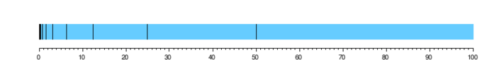
Zeno's Paradox: Say you are working from a location [latex]x=0[/latex] toward [latex]x=100[/latex]. Before you can get there, you must get halfway there. Before you can get halfway there, you must get a quarter of the way there. Before traveling a quarter, you must travel one-eighth; before an eighth, one-sixteenth; and so on.
Definition
For any sequence of rational numbers, real numbers, complex numbers, functions thereof, etc., the associated series is defined as the ordered formal sum: [latex-display]\displaystyle{\sum_{n=0}^{\infty}a_n = a_0 + a_1 + a_2 + \cdots}[/latex-display] The sequence of partial sums [latex]\{S_k\}[/latex] associated to a series [latex]\sum_{n=0}^\infty a_n[/latex] is defined for each k as the sum of the sequence [latex]\{a_n\}[/latex] from [latex]a_0[/latex] to [latex]a_k[/latex]: [latex-display]\displaystyle{S_k = \sum_{n=0}^{k}a_n = a_0 + a_1 + \cdots + a_k}[/latex-display] By definition, the series [latex]\sum_{n=0}^{\infty} a_n[/latex] converges to a limit [latex]L[/latex] if and only if the associated sequence of partial sums [latex]\{S_k\}[/latex] converges to [latex]L[/latex]. This definition is usually written as follows: [latex-display]\displaystyle{L = \sum_{n=0}^{\infty}a_n \Leftrightarrow L = \lim_{k \rightarrow \infty} S_k}[/latex-display]The Integral Test and Estimates of Sums
The integral test is a method of testing infinite series of nonnegative terms for convergence by comparing them to an improper integral.Learning Objectives
Describe the purpose of the integral testKey Takeaways
Key Points
- The integral test uses a monotonically decreasing function [latex]f[/latex] defined on the unbounded interval [latex][N, \infty)[/latex] (where [latex]N[/latex] is an integer).
- The infinite series [latex]\sum_{n=N}^\infty f(n)[/latex] converges to a real number if and only if the improper integral [latex]\int_N^\infty f(x)\,dx[/latex] is finite. In other words, if the integral diverges, then the series diverges as well.
- Integral tests proves that the harmonic series [latex]\sum_{n=1}^\infty \frac1n[/latex] diverges.
Key Terms
- improper integral: an integral where at least one of the endpoints is taken as a limit, either to a specific number or to infinity
- natural logarithm: the logarithm in base [latex]e[/latex]
Statement of the test
Consider an integer [latex]N[/latex] and a non-negative function [latex]f[/latex] defined on the unbounded interval [latex][N, \infty )[/latex], on which it is monotonically decreasing. The infinite series [latex]\sum_{n=N}^\infty f(n)[/latex] converges to a real number if and only if the improper integral [latex]\int_N^\infty f(x)\,dx[/latex] is finite. In other words, if the integral diverges, then the series diverges as well. Although we won't go into the details, the proof of the test also gives the lower and upper bounds: [latex-display]\displaystyle{\int_N^\infty f(x)\,dx\le\sum_{n=N}^\infty f(n)\le f(N)+\int_N^\infty f(x)\,dx}[/latex-display] for the infinite series.Applications
The harmonic series [latex]\sum_{n=1}^\infty \frac1n[/latex] diverges because, using the natural logarithm (its derivative) and the fundamental theorem of calculus, we get: [latex-display]\displaystyle{\int_1^M\frac1x\,dx=\ln x\Bigr|_1^M=\ln M\to\infty \quad\text{for }M\to\infty}[/latex-display] On the other hand, the series [latex]\sum_{n=1}^\infty \frac1{n^{1+\varepsilon}}[/latex] converges for every [latex]\varepsilon > 0[/latex] because, by the power rule: [latex-display]\displaystyle{\int_1^M\frac1{x^{1+\varepsilon}}\,dx =-\frac1{\varepsilon x^\varepsilon}\biggr|_1^M= \frac1\varepsilon\Bigl(1-\frac1{M^\varepsilon}\Bigr) \le\frac1\varepsilon }[/latex-display]
Integral Test: The integral test applied to the harmonic series. Since the area under the curve [latex]y = \frac{1}{x}[/latex] for [latex]x \in [1, \infty)[/latex] is infinite, the total area of the rectangles must be infinite as well.
Comparison Tests
Comparison test may mean either limit comparison test or direct comparison test, both of which can be used to test convergence of a series.Learning Objectives
Distinguish the limit comparison and the direct comparison testsKey Takeaways
Key Points
- For sequences [latex]\{a_n \}[/latex], [latex]\{b_n \}[/latex], both with non-negative terms only, if [latex]\lim_{n \to \infty} \frac{a_n}{b_n} = c[/latex] with [latex]0 < c < \infty[/latex].
- If the infinite series [latex]\sum b_n[/latex] converges and [latex]0 \le a_n \le b_n[/latex] for all sufficiently large [latex]n[/latex] (that is, for all [latex]n > N[/latex] for some fixed value [latex]N[/latex]), then the infinite series [latex]\sum a_n[/latex] also converges.
- If the infinite series [latex]\sum b_n[/latex] diverges and [latex]0 \le a_n \le b_n[/latex] for all sufficiently large [latex]n[/latex], then the infinite series [latex]\sum a_n[/latex] also diverges.
Key Terms
- integral test: a method used to test infinite series of non-negative terms for convergence by comparing it to improper integrals
- improper integral: an integral where at least one of the endpoints is taken as a limit, either to a specific number or to infinity
Limit Comparison Test
Statement: Suppose that we have two series, [latex]\Sigma_n a_n[/latex] and [latex]\Sigma_n b_n[/latex], where [latex]a_n[/latex], [latex]b_n[/latex] are greater than or equal to [latex]0[/latex] for all [latex]n[/latex]. If [latex]\lim_{n \to \infty} \frac{a_n}{b_n} = c[/latex] with [latex]0 < c < \infty[/latex], then either both series converge or both series diverge. Example: We want to determine if the series [latex]\Sigma \frac{n+1}{2n^2}[/latex] converges or diverges. For this we compare it with the series [latex]\Sigma \frac{1}{n}[/latex], which diverges. As [latex]\lim_{n \to \infty} \frac{n+1}{2n^2} \frac{n}{1} = \frac{1}{2}[/latex], we have that the original series also diverges.
Limit Convergence Test: The ratio between [latex]\frac{n+1}{2n^2}[/latex] and [latex]\frac{1}{n}[/latex] for [latex]n \rightarrow ∞[/latex] is [latex]\frac{1}{2}[/latex]. Since the sum of the sequence [latex]\frac{1}{n}[/latex] [latex]\left ( \text{i.e., }\sum {\frac{1}{n}}\right)[/latex] diverges, the limit convergence test tells that the original series (with [latex]\frac{n+1}{2n^2}[/latex]) also diverges.
Direct Comparison Test
The direct comparison test provides a way of deducing the convergence or divergence of an infinite series or an improper integral. In both cases, the test works by comparing the given series or integral to one whose convergence properties are known. In this atom, we will check the series case only. For sequences [latex]\{a_n\}[/latex], [latex]\{b_n\}[/latex] with non-negative terms:- If the infinite series [latex]\sum b_n[/latex] converges and [latex]0 \le a_n \le b_n[/latex] for all sufficiently large [latex]n[/latex] (that is, for all [latex]n>N[/latex] for some fixed value [latex]N[/latex]), then the infinite series [latex]\sum a_n[/latex] also converges.
- If the infinite series [latex]\sum b_n[/latex] diverges and [latex]a_n \ge b_n \ge 0[/latex] for all sufficiently large [latex]n[/latex], then the infinite series [latex]\sum a_n[/latex] also diverges.
Example
The series [latex]\Sigma \frac{1}{n^3 + 2n}[/latex] converges because [latex]\frac{1}{n^3 + 2n} < \frac{1}{n^3}[/latex] for [latex]n > 0[/latex] and [latex]\Sigma \frac{1}{n^3}[/latex] converges.Alternating Series
An alternating series is an infinite series of the form [latex]\sum_{n=0}^\infty (-1)^n\,a_n[/latex] or [latex]\sum_{n=0}^\infty (-1)^{n-1}\,a_n[/latex] with [latex]a_n > 0[/latex] for all [latex]n[/latex].Learning Objectives
Describe the properties of an alternating series and the requirements for one to convergeKey Takeaways
Key Points
- The theorem known as the "Leibniz Test," or the alternating series test, tells us that an alternating series will converge if the terms [latex]a_n[/latex] converge to [latex]0[/latex] monotonically.
- The signs of the general terms alternate between positive and negative.
- The sum [latex]\sum_{n=1}^\infty \frac{(-1)^{n+1}}{n}[/latex] converges by the alternating series test.
Key Terms
- monotone: property of a function to be either always decreasing or always increasing
- Cauchy sequence: a sequence whose elements become arbitrarily close to each other as the sequence progresses
Alternating Series Test
The theorem known as the "Leibniz Test," or the alternating series test, tells us that an alternating series will converge if the terms [latex]a_n[/latex] converge to [latex]0[/latex] monotonically. Proof: Suppose the sequence [latex]a_n[/latex] converges to [latex]0[/latex] and is monotone decreasing. If [latex]m[/latex] is odd and [latex]S_m - S_n < a_{m}[/latex] via the following calculation: [latex-display]\begin{align} S_m - S_n & = \sum_{k=0}^m(-1)^k\,a_k\,-\,\sum_{k=0}^n\,(-1)^k\,a_k\ \\& = \sum_{k=m+1}^n\,(-1)^k\,a_k \\ & =a_{m+1}-a_{m+2}+a_{m+3}-a_{m+4}+\cdots+a_n\\ & =\displaystyle a_{m+1}-(a_{m+2}-a_{m+3}) -\cdots-a_n \le a_{m+1}\le a_{m} \\& \quad [a_{n} \text{ decreasing}]. \end{align}[/latex-display] Since [latex]a_n[/latex] is monotonically decreasing, the terms are negative. Thus, we have the final inequality [latex]S_m - S_n \le a_{m}[/latex]. Similarly, it can be shown that, since [latex]a_m[/latex] converges to [latex]0[/latex], [latex]S_m - S_n[/latex] converges to [latex]0[/latex] for [latex]m, n \rightarrow \infty[/latex]. Therefore, our partial sum [latex]S_m[/latex] converges. (The sequence [latex]\{ S_m \}[/latex] is said to form a Cauchy sequence, meaning that elements of the sequence become arbitrarily close to each other as the sequence progresses.) The argument for [latex]m[/latex] even is similar. Example: [latex-display]\displaystyle{\sum_{n=1}^\infty \frac{(-1)^{n+1}}{n} = 1 - \frac{1}{2} + \frac{1}{3} - \frac{1}{4} + \cdots}[/latex-display] [latex]a_n = \frac1n[/latex] converges to 0 monotonically. Therefore, the sum [latex]\sum_{n=1}^\infty \frac{(-1)^{n+1}}{n}[/latex] converges by the alternating series test.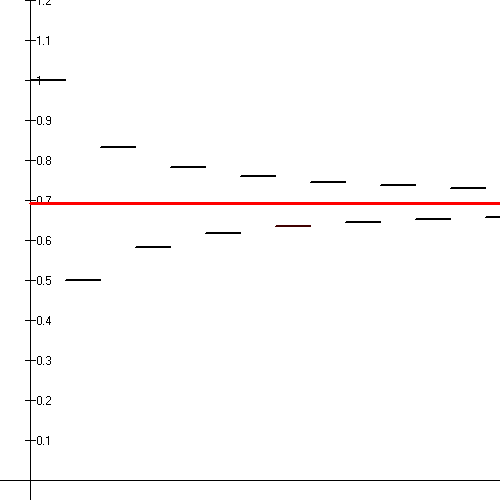
Alternating Harmonic Series: The first fourteen partial sums of the alternating harmonic series (black line segments) shown converging to the natural logarithm of 2 (red line).
Absolute Convergence and Ratio and Root Tests
An infinite series of numbers is said to converge absolutely if the sum of the absolute value of the summand is finite.Learning Objectives
State the conditions when an infinite series of numbers converge absolutelyKey Takeaways
Key Points
- A real or complex series [latex]\textstyle\sum_{n=0}^\infty a_n[/latex] is said to converge absolutely if [latex]\textstyle\sum_{n=0}^\infty \left|a_n\right| = L[/latex] for some real number [latex]L[/latex].
- The root test is a convergence test of an infinite series that makes use of the limit [latex]L = \lim_{n\rightarrow\infty}\left|\frac{a_{n+1}}{a_n}\right|[/latex].
- The root test is a criterion for the convergence of an infinite series using the limit superior [latex]C = \limsup_{n\rightarrow\infty}\sqrt[n]{|a_n|}[/latex].
Key Terms
- summand: something which is added or summed
- improper integral: an integral where at least one of the endpoints is taken as a limit, either to a specific number or to infinity
- limit superior: the supremum of the set of accumulation points of a given sequence or set
Ratio Test
The ratio test is a test (or "criterion") for the convergence of a series [latex]\sum_{n=1}^\infty a_n[/latex], where each term is a real or complex number and [latex]a_n[/latex] is nonzero when n is large. The test was first published by Jean le Rond d'Alembert and is sometimes known as d'Alembert's ratio test. The usual form of the test makes use of the limit, [latex]L = \lim_{n\rightarrow\infty}\left|\frac{a_{n+1}}{a_n}\right|[/latex]. The ratio test states that,- if [latex]L < 1[/latex], then the series converges absolutely;
- if [latex]L > 1[/latex], then the series does not converge;
- if [latex]L = 1[/latex] or the limit fails to exist, then the test is inconclusive, because there exist both convergent and divergent series that satisfy this case.
Root Test
The root test is a criterion for the convergence (a convergence test) of an infinite series. It depends on the quantity [latex]\limsup_{n\rightarrow\infty}\sqrt[n]{|a_n|}[/latex], where [latex]a_n[/latex] are the terms of the series, and states that the series converges absolutely if this quantity is less than one but diverges if it is greater than one. It is particularly useful in connection with power series. The root test was developed first by Augustin-Louis Cauchy and so is sometimes known as the Cauchy root test, or Cauchy's radical test. For a series [latex]\sum_{n=1}^\infty a_n[/latex], the root test uses the number [latex]C = \limsup_{n\rightarrow\infty}\sqrt[n]{ \left|a_n \right|}[/latex], where "lim sup" denotes the limit superior, possibly ∞. Note that if [latex]\lim_{n\rightarrow\infty}\sqrt[n]{ \left|a_n \right|}[/latex] converges, then it equals [latex]C[/latex] and may be used in the root test instead. The root test states that- if [latex]C < 1[/latex], then the series converges absolutely;
- if [latex]C > 1[/latex], then the series diverges;
- if [latex]C = 1[/latex] and the limit approaches strictly from above, then the series diverges;
- otherwise the test is inconclusive (the series may diverge, converge absolutely, or converge conditionally).

Ratio Test: In this example, the ratio of adjacent terms in the blue sequence converges to [latex]L=\frac{1}{2}[/latex]. We choose [latex]r = \frac{L+1}{2} = \frac{3}{4}[/latex]. Then the blue sequence is dominated by the red sequence for all [latex]n \geq 2[/latex]. The red sequence converges, so the blue sequence does as well.
Tips for Testing Series
Convergence tests are methods of testing for the convergence or divergence of an infinite series.Learning Objectives
Formulate three techniques that will help when testing the convergence of a seriesKey Takeaways
Key Points
- There is no single convergence test which works for all series out there.
- Practice and training will help you choose the right test for a given series.
- We have learned about the root /ratio test, integral test, and direct/ limit comparison test.
Key Terms
- conditional convergence: A series or integral is said to be conditionally convergent if it converges but does not converge absolutely.
List of Tests
Limit of the Summand: If the limit of the summand is undefined or nonzero, then the series must diverge. Ratio test: For [latex]r = \lim_{n \to \infty} \left|\frac{a_{n+1}}{a_n}\right|[/latex], if [latex]r < 1[/latex], the series converges; if [latex]r > 1[/latex], the series diverges; if [latex]r = 1[/latex], the test is inconclusive. Root test: For [latex]r = \limsup_{n \to \infty}\sqrt[n]{ \left|a_n \right|}[/latex], if [latex]r < 1[/latex], then the series converges; if [latex]r > 1[/latex], then the series diverges; if [latex]r = 1[/latex], the root test is inconclusive. Integral test: For a positive, monotone decreasing function [latex]f(x)[/latex] such that [latex]f(n)=a_n[/latex], if [latex]\int_{1}^{\infty} f(x)\, dx = \lim_{t \to \infty} \int_{1}^{t} f(x)\, dx < \infty[/latex] then the series converges. But if the integral diverges, then the series does so as well.
Integral Test: The integral test applied to the harmonic series. Since the area under the curve [latex]y = \frac{1}{x}[/latex] for [latex]x \in [1, ∞)[/latex] is infinite, the total area of the rectangles must be infinite as well.
Power Series
A power series (in one variable) is an infinite series of the form [latex]f(x) = \sum_{n=0}^\infty a_n \left( x-c \right)^n[/latex], where [latex]a_n[/latex] is the coefficient of the [latex]n[/latex]th term and [latex]x[/latex] varies around [latex]c[/latex].Learning Objectives
Express a power series in a general formKey Takeaways
Key Points
- Power series usually arise as the Taylor series of some known function.
- In many situations [latex]c[/latex] is equal to zero—for instance, when considering a Maclaurin series. In such cases, the power series takes the simpler form [latex]f(x) = \sum_{n=0}^\infty a_n x^n = a_0 + a_1 x + a_2 x^2 + a_3 x^3 + \cdots[/latex].
- A power series will converge for some values of the variable [latex]x[/latex] and may diverge for others. If there exists a number [latex]r[/latex] with [latex]0 < r \leq \infty[/latex] such that the series converges when [latex]\left| x-c \right| <r[/latex] and diverges when [latex]\left| x-c \right| >r[/latex], the number [latex]r[/latex] is called the radius of convergence of the power series.
Key Terms
- Z-transform: transform that converts a discrete time-domain signal into a complex frequency-domain representation
- combinatorics: a branch of mathematics that studies (usually finite) collections of objects that satisfy specified criteria and their structures
Exponential Function as a Power Series: The exponential function (in blue), and the sum of the first [latex]n+1[/latex] terms of its Maclaurin power series (in red).
Radius of Convergence
A power series will converge for some values of the variable [latex]x[/latex] and may diverge for others. All power series [latex]f(x)[/latex] in powers of [latex](x-c)[/latex] will converge at [latex]x=c[/latex]. If [latex]c[/latex] is not the only convergent point, then there is always a number [latex]r[/latex] with 0 < r ≤ ∞ such that the series converges whenever [latex]\left| x-c \right| <r[/latex] and diverges whenever [latex]\left| x-c \right| >r[/latex]. The number [latex]r[/latex] is called the radius of convergence of the power series. According to the Cauchy-Hadamard theorem, the radius [latex]r[/latex] can be computed from [latex-display]\displaystyle{r^{-1}=\lim_{n\to\infty}\left|{a_{n+1}\over a_n}\right|}[/latex-display] if this limit exists.Expressing Functions as Power Functions
A power function is a function of the form [latex]f(x) = cx^r[/latex] where [latex]c[/latex] and [latex]r[/latex] are constant real numbers.Learning Objectives
Describe the relationship between the power functions and infinitely differentiable functionsKey Takeaways
Key Points
- Since all infinitely differentiable functions can be represented in power series, any infinitely differentiable function can be represented as a sum of many power functions (of integer exponents ).
- Therefore, an arbitrary function that is infinitely differentiable is expressed as an infinite sum of power functions ([latex]x^n[/latex]) of integer exponent: [latex]f(x) = \sum_{n=0} ^ {\infty} \frac {f^{(n)}(0)}{n! } \, x^{n}[/latex].
- Functions of the form [latex]f(x) = x^{3}[/latex], [latex]f(x) = x^{1.2}[/latex], [latex]f(x) = x^{-4}[/latex] are all power functions.
Key Terms
- differentiable: having a derivative, said of a function whose domain and co-domain are manifolds
- power law: any of many mathematical relationships in which something is related to something else by an equation of the form [latex]f(x) = a x^k[/latex]

[latex]\sin x[/latex] in Taylor Approximations: Figure shows [latex]\sin x[/latex] and Taylor approximations, polynomials of degree 1, 3, 5, 7, 9, 11 and 13. As more power functions with larger exponents are added, the Taylor polynomial approaches the correct function.
Examples
Functions of the form [latex]f(x) = x^3[/latex], [latex]f(x) = x^{1.2}[/latex], [latex]f(x) = x^{-4}[/latex] are all power functions.Taylor and Maclaurin Series
Taylor series represents a function as an infinite sum of terms calculated from the values of the function's derivatives at a single point.Learning Objectives
Identify a Maclaurin series as a special case of a Taylor seriesKey Takeaways
Key Points
- Any finite number of initial terms of the Taylor series of a function is called a Taylor polynomial.
- A function that is equal to its Taylor series in an open interval (or a disc in the complex plane) is known as an analytic function.
- The Taylor series of a real or complex-valued function [latex]f(x)[/latex] that is infinitely differentiable in a neighborhood of a real or complex number a is the power series [latex]f(x)=∑∞n=0f(n)(a)n!(x−a)nf(x) = \sum_{n=0} ^ {\infty} \frac {f^{(n)}(a)}{n! } \, (x-a)^{n}[/latex]. If [latex]a = 0[/latex], the series is called a Maclaurin series.
Key Terms
- differentiable: having a derivative, said of a function whose domain and co-domain are manifolds
- analytic function: a real valued function which is uniquely defined through its derivatives at one point
Exponential Function as a Power Series: The exponential function (in blue) and the sum of the first [latex]n+1[/latex] terms of its Taylor series at [latex]0[/latex] (in red) up to [latex]n=8[/latex].
Example 1
The Maclaurin series for [latex](1 − x)^{−1}[/latex] for [latex]\left| x \right| < 1[/latex] is the geometric series: [latex]1+x+x^2+x^3+\cdots\![/latex] so the Taylor series for [latex]x^{−1}[/latex] at [latex]a=1[/latex] is: [latex-display]1-(x-1)+(x-1)^2-(x-1)^3+\cdots[/latex-display]Example 2
The Taylor series for the exponential function [latex]e^x[/latex] at [latex]a=0[/latex] is: [latex-display]\displaystyle{1 + \frac{x^1}{1! } + \frac{x^2}{2! } + \frac{x^3}{3! } + \frac{x^4}{4! } + \frac{x^5}{5! }+ \cdots \\= 1 + x + \frac{x^2}{2} + \frac{x^3}{6} + \frac{x^4}{24} + \frac{x^5}{120} + \cdots\! \\= \sum_{n=0}^\infty \frac{x^n}{n! }}[/latex-display]Applications of Taylor Series
Taylor series expansion can help approximating values of functions and evaluating definite integrals.Learning Objectives
Describe applications of the Taylor series expansionKey Takeaways
Key Points
- The partial sums of the series, which is called the Taylor polynomials, can be used as approximations of the entire function.
- Differentiation and integration of power series can be performed term by term, and hence could be easier than directly working with the original function.
- The (truncated) series can be used to compute function values numerically. This is particularly useful in evaluating special mathematical functions (such as Bessel function).
Key Terms
- definite integral: the integral of a function between an upper and lower limit
- complex analysis: theory of functions of a complex variable; a branch of mathematical analysis that investigates functions of complex numbers
- analytic function: a real valued function which is uniquely defined through its derivatives at one point
Taylor Polynomials: As more terms are added to the Taylor polynomial, it approaches the correct function. This image shows [latex]\sin x[/latex] and its Taylor approximations, polynomials of degree 1, 3, 5, 7, 9, 11 and 13.
Summing an Infinite Series
Infinite sequences and series can either converge or diverge.Learning Objectives
Describe properties of the infinite seriesKey Takeaways
Key Points
- Infinite sequences and series continue indefinitely.
- A series is said to converge when the sequence of partial sums has a finite limit.
- A series is said to diverge when the limit is infinite or does not exist.
Key Terms
- limit: a value to which a sequence or function converges
- sequence: an ordered list of objects

Infinite Series: An infinite sequence of real numbers shown in blue dots. This sequence is neither increasing, nor decreasing, nor convergent, nor Cauchy. It is, however, bounded.
Convergence of Series with Positive Terms
For a sequence [latex]\{a_n\}[/latex], where [latex]a_n[/latex] is a non-negative real number for every [latex]n[/latex], the sum [latex]\sum_{n=0}^{\infty}a_n[/latex] can either converge or diverge to [latex]\infty[/latex].Learning Objectives
Identify convergence conditions for a sequence with positive termsKey Takeaways
Key Points
- Because the partial sum [latex]S_k[/latex] of a series with non-negative terms can only increase as [latex]k[/latex] becomes larger, the limit of the partial sum can either converge or diverge to [latex]\infty[/latex].
- A geometric sum [latex]1 + \frac{1}{2}+ \frac{1}{4}+ \frac{1}{8}+\cdots+ \frac{1}{2^n}+\cdots[/latex] converges to [latex]2[/latex], which can be understood visually.
- The series [latex]\sum_{n \ge 1} \frac{1}{n^2}[/latex] is convergent. This can be seen by comparing individual terms of the series with a sequence [latex]\left( b_n = \frac{1}{n-1} - \frac{1}{n} \right)[/latex], which is know to converge.
Key Terms
- converge: of a sequence, to have a limit
- convergence test: methods of testing for the convergence, conditional convergence, absolute convergence, interval of convergence, or divergence of an infinite series
Example 1
The series [latex]\sum_{n \ge 1} \frac{1}{n^2}[/latex] is convergent because of the inequality: [latex-display]\displaystyle{\frac1 {n^2} \le \frac{1}{n-1} - \frac{1}{n}, (n \ge 2)}[/latex-display] and because: [latex-display]\displaystyle{\sum_{n \ge 2} \left(\frac{1}{n-1} - \frac{1}{n} \right) =\left(1-\frac{1}{2}\right) + \left(\frac{1}{2}-\frac{1}{3}\right) + \left(\frac{1}{3}-\frac{1}{4}\right) + \cdots = 1}[/latex-display]Example 2
Would the series [latex-display]\displaystyle{S = 1 + \frac{1}{2}+ \frac{1}{4}+ \frac{1}{8}+\cdots+ \frac{1}{2^n}+\cdots}[/latex-display] converge? It is possible to "visualize" its convergence on the real number line? We can imagine a line of length [latex]2[/latex], with successive segments marked off of lengths [latex]1[/latex], [latex]\frac{1}{2}[/latex], [latex]\frac{1}{4}[/latex], etc. There is always room to mark the next segment, because the amount of line remaining is always the same as the last segment marked: when we have marked off [latex]\frac{1}{2}[/latex], we still have a piece of length [latex]\frac{1}{2}[/latex] unmarked, so we can certainly mark the next [latex]\frac{1}{4}[/latex]. This argument does not prove that the sum is equal to [latex]2[/latex] (although it is), but it does prove that it is at most [latex]2[/latex]. In other words, the series has an upper bound. Proving that the series is equal to [latex]2[/latex] requires only elementary algebra, however. If the series is denoted [latex]S[/latex], it can be seen that: [latex-display]\displaystyle{\frac{S}{2} \,= \frac{1+ \frac{1}{2}+ \frac{1}{4}+ \frac{1}{8}+\cdots}{2} \\ \quad= \frac{1}{2}+ \frac{1}{4}+ \frac{1}{8}+ \frac{1}{16} +\cdots}[/latex-display] Therefore: [latex-display]\displaystyle{S-\frac{S}{2} = 1\\S = 2}[/latex-display]
Geometric Sum: Visualization of the geometric sum in Example 2. The length of the line ([latex]2[/latex]) can contain all the successive segments marked off of lengths [latex]1[/latex], [latex]\frac{1}{2}[/latex], [latex]\frac{1}{4}[/latex], etc.
Licenses & Attributions
CC licensed content, Shared previously
- Curation and Revision. Provided by: Boundless.com License: CC BY-SA: Attribution-ShareAlike.
CC licensed content, Specific attribution
- Sequence. Provided by: Wikipedia Located at: https://en.wikipedia.org/wiki/Sequence. License: CC BY-SA: Attribution-ShareAlike.
- recursion. Provided by: Wiktionary License: CC BY-SA: Attribution-ShareAlike.
- set. Provided by: Wiktionary License: CC BY-SA: Attribution-ShareAlike.
- Sequence. Provided by: Wikipedia License: CC BY: Attribution.
- Series (mathematics). Provided by: Wikipedia License: CC BY-SA: Attribution-ShareAlike.
- Zeno's dichotomy. Provided by: Wikipedia License: CC BY-SA: Attribution-ShareAlike.
- sequence. Provided by: Wiktionary License: CC BY-SA: Attribution-ShareAlike.
- Sequence. Provided by: Wikipedia License: CC BY: Attribution.
- Zeno's paradoxes. Provided by: Wikipedia License: CC BY: Attribution.
- Integral test for convergence. Provided by: Wikipedia License: CC BY-SA: Attribution-ShareAlike.
- natural logarithm. Provided by: Wiktionary License: CC BY-SA: Attribution-ShareAlike.
- improper integral. Provided by: Wiktionary License: CC BY-SA: Attribution-ShareAlike.
- Sequence. Provided by: Wikipedia License: CC BY: Attribution.
- Zeno's paradoxes. Provided by: Wikipedia License: CC BY: Attribution.
- Integral test for convergence. Provided by: Wikipedia License: CC BY: Attribution.
- Limit comparison test. Provided by: Wikipedia License: CC BY-SA: Attribution-ShareAlike.
- Direct comparison test. Provided by: Wikipedia License: CC BY-SA: Attribution-ShareAlike.
- Boundless. Provided by: Boundless Learning License: CC BY-SA: Attribution-ShareAlike.
- improper integral. Provided by: Wiktionary Located at: https://en.wiktionary.org/wiki/improper_integral. License: CC BY-SA: Attribution-ShareAlike.
- Sequence. Provided by: Wikipedia License: CC BY: Attribution.
- Zeno's paradoxes. Provided by: Wikipedia License: CC BY: Attribution.
- Integral test for convergence. Provided by: Wikipedia License: CC BY: Attribution.
- Sequence. Provided by: Wikipedia License: CC BY: Attribution.
- Alternating series. Provided by: Wikipedia License: CC BY-SA: Attribution-ShareAlike.
- Cauchy sequence. Provided by: Wikipedia License: CC BY-SA: Attribution-ShareAlike.
- monotone. Provided by: Wiktionary License: CC BY-SA: Attribution-ShareAlike.
- Sequence. Provided by: Wikipedia License: CC BY: Attribution.
- Zeno's paradoxes. Provided by: Wikipedia License: CC BY: Attribution.
- Integral test for convergence. Provided by: Wikipedia License: CC BY: Attribution.
- Sequence. Provided by: Wikipedia License: CC BY: Attribution.
- Harmonic series (mathematics). Provided by: Wikipedia License: CC BY: Attribution.
- Ratio test. Provided by: Wikipedia License: CC BY-SA: Attribution-ShareAlike.
- Absolute convergence. Provided by: Wikipedia License: CC BY-SA: Attribution-ShareAlike.
- Root test. Provided by: Wikipedia License: CC BY-SA: Attribution-ShareAlike.
- summand. Provided by: Wiktionary License: CC BY-SA: Attribution-ShareAlike.
- improper integral. Provided by: Wiktionary License: CC BY-SA: Attribution-ShareAlike.
- limit superior. Provided by: Wiktionary License: CC BY-SA: Attribution-ShareAlike.
- Sequence. Provided by: Wikipedia License: CC BY: Attribution.
- Zeno's paradoxes. Provided by: Wikipedia License: CC BY: Attribution.
- Integral test for convergence. Provided by: Wikipedia License: CC BY: Attribution.
- Sequence. Provided by: Wikipedia License: CC BY: Attribution.
- Harmonic series (mathematics). Provided by: Wikipedia License: CC BY: Attribution.
- Ratio test proof. Provided by: Wikipedia License: CC BY-SA: Attribution-ShareAlike.
- Convergence tests. Provided by: Wikipedia License: CC BY-SA: Attribution-ShareAlike.
- conditional convergence. Provided by: Wikipedia License: CC BY-SA: Attribution-ShareAlike.
- Sequence. Provided by: Wikipedia License: CC BY: Attribution.
- Zeno's paradoxes. Provided by: Wikipedia License: CC BY: Attribution.
- Integral test for convergence. Provided by: Wikipedia License: CC BY: Attribution.
- Sequence. Provided by: Wikipedia License: CC BY: Attribution.
- Harmonic series (mathematics). Provided by: Wikipedia Located at: https://en.wikipedia.org/wiki/Harmonic_series_(mathematics). License: CC BY: Attribution.
- Ratio test proof. Provided by: Wikipedia License: CC BY-SA: Attribution-ShareAlike.
- Integral test for convergence. Provided by: Wikipedia License: CC BY: Attribution.
- Power series. Provided by: Wikipedia License: CC BY-SA: Attribution-ShareAlike.
- combinatorics. Provided by: Wiktionary License: CC BY-SA: Attribution-ShareAlike.
- Z-transform. Provided by: Wiktionary License: CC BY-SA: Attribution-ShareAlike.
- Sequence. Provided by: Wikipedia License: CC BY: Attribution.
- Zeno's paradoxes. Provided by: Wikipedia License: CC BY: Attribution.
- Integral test for convergence. Provided by: Wikipedia License: CC BY: Attribution.
- Sequence. Provided by: Wikipedia License: CC BY: Attribution.
- Harmonic series (mathematics). Provided by: Wikipedia License: CC BY: Attribution.
- Ratio test proof. Provided by: Wikipedia License: CC BY-SA: Attribution-ShareAlike.
- Integral test for convergence. Provided by: Wikipedia License: CC BY: Attribution.
- Power series. Provided by: Wikipedia License: CC BY: Attribution.
- Taylor series. Provided by: Wikipedia License: CC BY-SA: Attribution-ShareAlike.
- Power function. Provided by: Wikipedia License: CC BY-SA: Attribution-ShareAlike.
- differentiable. Provided by: Wiktionary License: CC BY-SA: Attribution-ShareAlike.
- power law. Provided by: Wiktionary License: CC BY-SA: Attribution-ShareAlike.
- Sequence. Provided by: Wikipedia License: CC BY: Attribution.
- Zeno's paradoxes. Provided by: Wikipedia License: CC BY: Attribution.
- Integral test for convergence. Provided by: Wikipedia License: CC BY: Attribution.
- Sequence. Provided by: Wikipedia License: CC BY: Attribution.
- Harmonic series (mathematics). Provided by: Wikipedia License: CC BY: Attribution.
- Ratio test proof. Provided by: Wikipedia License: CC BY-SA: Attribution-ShareAlike.
- Integral test for convergence. Provided by: Wikipedia License: CC BY: Attribution.
- Power series. Provided by: Wikipedia License: CC BY: Attribution.
- Taylor series. Provided by: Wikipedia License: CC BY: Attribution.
- Taylor series. Provided by: Wikipedia License: CC BY-SA: Attribution-ShareAlike.
- differentiable. Provided by: Wiktionary License: CC BY-SA: Attribution-ShareAlike.
- analytic function. Provided by: Wiktionary License: CC BY-SA: Attribution-ShareAlike.
- Sequence. Provided by: Wikipedia License: CC BY: Attribution.
- Zeno's paradoxes. Provided by: Wikipedia License: CC BY: Attribution.
- Integral test for convergence. Provided by: Wikipedia License: CC BY: Attribution.
- Sequence. Provided by: Wikipedia License: CC BY: Attribution.
- Harmonic series (mathematics). Provided by: Wikipedia License: CC BY: Attribution.
- Ratio test proof. Provided by: Wikipedia License: CC BY-SA: Attribution-ShareAlike.
- Integral test for convergence. Provided by: Wikipedia License: CC BY: Attribution.
- Power series. Provided by: Wikipedia Located at: https://en.wikipedia.org/wiki/Power_series. License: CC BY: Attribution.
- Taylor series. Provided by: Wikipedia License: CC BY: Attribution.
- Taylor series. Provided by: Wikipedia License: CC BY: Attribution.
- Taylor series. Provided by: Wikipedia License: CC BY-SA: Attribution-ShareAlike.
- complex analysis. Provided by: Wikipedia License: CC BY-SA: Attribution-ShareAlike.
- definite integral. Provided by: Wiktionary License: CC BY-SA: Attribution-ShareAlike.
- analytic function. Provided by: Wiktionary License: CC BY-SA: Attribution-ShareAlike.
- Sequence. Provided by: Wikipedia License: CC BY: Attribution.
- Zeno's paradoxes. Provided by: Wikipedia License: CC BY: Attribution.
- Integral test for convergence. Provided by: Wikipedia License: CC BY: Attribution.
- Sequence. Provided by: Wikipedia License: CC BY: Attribution.
- Harmonic series (mathematics). Provided by: Wikipedia License: CC BY: Attribution.
- Ratio test proof. Provided by: Wikipedia License: CC BY-SA: Attribution-ShareAlike.
- Integral test for convergence. Provided by: Wikipedia License: CC BY: Attribution.
- Power series. Provided by: Wikipedia License: CC BY: Attribution.
- Taylor series. Provided by: Wikipedia License: CC BY: Attribution.
- Taylor series. Provided by: Wikipedia License: CC BY: Attribution.
- Taylor series. Provided by: Wikipedia License: CC BY: Attribution.
- Infinite series. Provided by: Wikipedia License: CC BY-SA: Attribution-ShareAlike.
- Series (mathematics). Provided by: Wikipedia License: CC BY-SA: Attribution-ShareAlike.
- limit. Provided by: Wiktionary License: CC BY-SA: Attribution-ShareAlike.
- sequence. Provided by: Wiktionary License: CC BY-SA: Attribution-ShareAlike.
- Sequence. Provided by: Wikipedia License: CC BY: Attribution.
- Zeno's paradoxes. Provided by: Wikipedia License: CC BY: Attribution.
- Integral test for convergence. Provided by: Wikipedia License: CC BY: Attribution.
- Sequence. Provided by: Wikipedia License: CC BY: Attribution.
- Harmonic series (mathematics). Provided by: Wikipedia License: CC BY: Attribution.
- Ratio test proof. Provided by: Wikipedia License: CC BY-SA: Attribution-ShareAlike.
- Integral test for convergence. Provided by: Wikipedia License: CC BY: Attribution.
- Power series. Provided by: Wikipedia License: CC BY: Attribution.
- Taylor series. Provided by: Wikipedia License: CC BY: Attribution.
- Taylor series. Provided by: Wikipedia License: CC BY: Attribution.
- Taylor series. Provided by: Wikipedia License: CC BY: Attribution.
- Sequence. Provided by: Wikipedia License: CC BY: Attribution.
- Series (mathematics). Provided by: Wikipedia License: CC BY-SA: Attribution-ShareAlike.
- convergence test. Provided by: Wikipedia License: CC BY-SA: Attribution-ShareAlike.
- converge. Provided by: Wiktionary License: CC BY-SA: Attribution-ShareAlike.
- Sequence. Provided by: Wikipedia License: CC BY: Attribution.
- Zeno's paradoxes. Provided by: Wikipedia Located at: https://en.wikipedia.org/wiki/Zeno%27s_paradoxes. License: CC BY: Attribution.
- Integral test for convergence. Provided by: Wikipedia License: CC BY: Attribution.
- Sequence. Provided by: Wikipedia License: CC BY: Attribution.
- Harmonic series (mathematics). Provided by: Wikipedia License: CC BY: Attribution.
- Ratio test proof. Provided by: Wikipedia License: CC BY-SA: Attribution-ShareAlike.
- Integral test for convergence. Provided by: Wikipedia License: CC BY: Attribution.
- Power series. Provided by: Wikipedia License: CC BY: Attribution.
- Taylor series. Provided by: Wikipedia License: CC BY: Attribution.
- Taylor series. Provided by: Wikipedia License: CC BY: Attribution.
- Taylor series. Provided by: Wikipedia License: CC BY: Attribution.
- Sequence. Provided by: Wikipedia License: CC BY: Attribution.
- Zeno's paradoxes. Provided by: Wikipedia License: CC BY: Attribution.
