Derivatives
The Derivative and Tangent Line Problem
The use of differentiation makes it possible to solve the tangent line problem by finding the slope [latex]f'(a)[/latex].Learning Objectives
Define a derivative as the slope of the tangent line to a point on a curveKey Takeaways
Key Points
- The tangent line [latex]t[/latex] (or simply the tangent) to a plane curve at a given point is the straight line that "just touches" the curve at that point.
- A straight line is said to be a tangent of a curve [latex]y=f(x)[/latex] at a point [latex]x = c[/latex] on the curve if the line passes through the point [latex](c, f(c))[/latex] on the curve and has slope [latex]f'(c)[/latex] where [latex]f'[/latex] is the derivative of [latex]f[/latex].
- Using derivatives, the equation of the tangent line can be stated as follows: [latex]y = f(a) + f{(a)}'(x-a)[/latex].
Key Terms
- tangent: a line touching a curve at a single point without crossing it there
- secant: a line that intersects a curve at two or more points

Tangent to a Curve: The line shows the tangent to the curve at the point represented by the dot. It barely touches the curve and shows the rate of change slope at the point.
Derivatives and Rates of Change
Differentiation is a way to calculate the rate of change of one variable with respect to another.Learning Objectives
Describe the derivative as the change in [latex]y[/latex] over the change in [latex]x[/latex] at each point on a graphKey Takeaways
Key Points
- Historically, the primary motivation for the study of differentiation was the tangent line problem, which is the task of, for a given curve, finding the slope of the straight line that is tangent to that curve at a given point.
- If [latex]y[/latex] is a linear function of [latex]x[/latex], then [latex]m = \frac{\Delta y}{\Delta x}[/latex].
- The derivative measures the slope of a graph at each point.
Key Terms
- slope: also called gradient; slope or gradient of a line describes its steepness
Slope of a function: A function with the slope shown for a given point.
The Derivative as a Function
If every point of a function has a derivative, there is a derivative function sending the point [latex]a[/latex] to the derivative of [latex]f[/latex] at [latex]x = a[/latex]: [latex]f'(a)[/latex].Learning Objectives
Explain how the derivative acts as a "function of functions"Key Takeaways
Key Points
- The derivative is an operator whose domain is the set of all functions that have derivatives at every point of their domain and whose range is a set of functions.
- The function whose value at [latex]x=a[/latex] equals [latex]f′(a)[/latex] whenever [latex]f′(a)[/latex] is defined and elsewhere is undefined is also called the derivative of [latex]f[/latex].
- By the definition of the derivative function, [latex]D(f)(a) = f′(a)[/latex], where [latex]D[/latex] is an operator whose domain is the set of all functions that have derivatives at every point of their domain and whose range is a set of functions.
Key Terms
- range: the set of values (points) which a function can obtain
- domain: the set of all possible mathematical entities (points) where a given function is defined
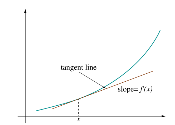
Derivative As Slope: The slope of tangent line shown represents the value of the derivative of the curved function at the point [latex]x[/latex].
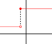
Discontinuous Function: At the point where the function makes a jump, the derivative of the function does not exist.
Differentiation Rules
The rules of differentiation can simplify derivatives by eliminating the need for complicated limit calculations.Learning Objectives
Practice using differentiation rules to simplify differentiating complicated expressionsKey Takeaways
Key Points
- Differentiation by polynomial expansion can be very complicated and prone to errors.
- Constant rule: if [latex]f(x)[/latex] is a constant, then its derivative, [latex]f'(x)[/latex], is [latex]0[/latex].
- Chain Rule: If [latex]f(x) = h(g(x))[/latex], then [latex]f'(x) = h'(g(x)) g'(x)[/latex].
- Product Rule: [latex](fg)' = f'g + g'f[/latex].
- Quotient Rule: [latex]\left ( \frac {f}{g} \right )' = \frac {f'g - fg'}{g^2}[/latex].
Key Terms
- difference quotient: the function difference [latex]\Delta F[/latex] divided by the point difference [latex]\Delta x[/latex]: [latex]\Delta F(x) / \Delta x[/latex]
- polynomial: an expression consisting of a sum of a finite number of terms, each term being the product of a constant coefficient and one or more variables raised to a non-negative integer power
The Constant Rule
If [latex]f(x)[/latex] is a constant, then [latex]f'(x) = 0[/latex], since the rate of change of a constant is always zero.The Sum Rule
[latex-display](\alpha f + \beta g)' = \alpha f' + \beta g'[/latex-display] for all functions [latex]f[/latex] and [latex]g[/latex] and all real numbers [latex]\alpha[/latex] and [latex]\beta[/latex].The Product Rule
[latex-display](fg)' = f'g + g'f[/latex-display] for all functions [latex]f[/latex] and [latex]g[/latex]. By extension, this means that the derivative of a constant times a function is the constant times the derivative of the function.The Quotient Rule
[latex-display]\displaystyle{\left ( \frac {f}{g} \right )' = \frac {f'g - fg'}{g^2}}[/latex-display] for all functions [latex]f[/latex] and [latex]g[/latex] at all inputs where [latex]g \neq 0[/latex].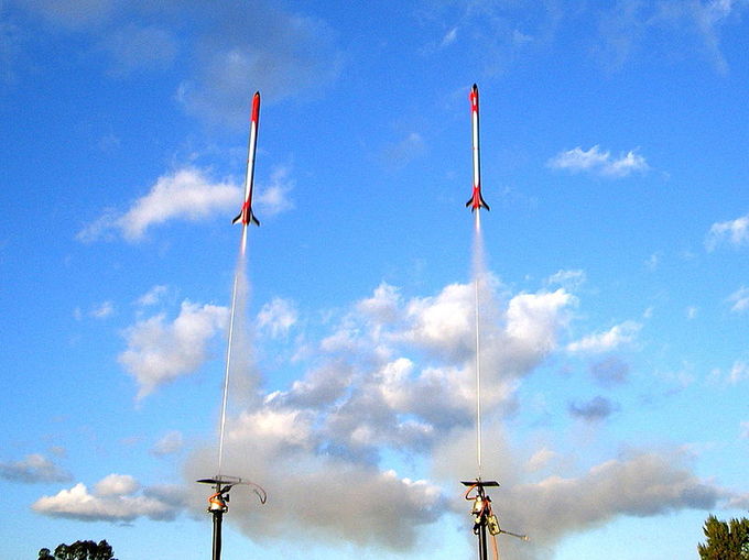
Model Rockets: The flight of model rockets can be modeled using the product rule.
The Chain Rule
If [latex]f(x) = h(g(x))[/latex], then [latex]f'(x) = h'(g(x)) g'(x)[/latex].Example
Consider the following function: [latex-display]f(x) = x^4 + e^{x^2} - ln(x)e^x + 7[/latex-display] Differentiating yields: [latex-display]\displaystyle{f'(x) = 4x^{(4-1)} + \frac{d(x^2)}{dx}e^{x^2} - \frac {d(ln\:x)}{dx}e^x - ln\:x\frac{d(e^x)}{dx} + 0 \\ \qquad = 4x^3 + 2xe^{x^2} - \frac {1}{x}e^x - ln(x)e^x}[/latex-display] Here the second term was computed using the chain rule and the third using the product rule. The known derivatives of the elementary functions [latex]x^2[/latex], [latex]x^4[/latex], [latex]\ln(x)[/latex], and [latex]e^x[/latex], as well as that of the constant 7, were also used.Derivatives of Trigonometric Functions
Derivatives of trigonometric functions can be found using the standard derivative formula.Learning Objectives
Identify the derivatives of the most common trigonometric functionsKey Takeaways
Key Points
- The derivative of the sine function is the cosine function.
- The derivative of the cosine function is the negative of the sine function.
- The derivative of the tangent function is the squared secant function.
Key Terms
- secant: a straight line that intersects a curve at two or more points
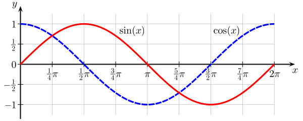
Sine and Cosine: In this image, one can see that where the line tangent to one curve has zero slope (the derivative of that curve is zero), the value of the other function is zero.
The Chain Rule
The chain rule is a formula for computing the derivative of the composition of two or more functions.Learning Objectives
Calculate the derivative of a composition of functions using the chain ruleKey Takeaways
Key Points
- If [latex]f[/latex] is a function and [latex]g[/latex] is a function, then the chain rule expresses the derivative of the composite function [latex]f \circ g[/latex] in terms of the derivatives of [latex]f[/latex] and [latex]g[/latex].
- The chain rule can be applied sequentially for as many functions as are nested inside one another.
- The chain rule for [latex]f \circ g(x)[/latex] is [latex]\frac{df}{dx} = \frac{df}{dg}\frac{dg}{dx}[/latex].
Key Terms
- composite: a function of a function

Skydiving: The path of a skydiver relies on many variables such as time and height. Use of the chain rule is needed for the complicated calculation.
Implicit Differentiation
Implicit differentiation makes use of the chain rule to differentiate implicitly defined functions.Learning Objectives
Use implicit differentiation to find the derivatives of functions that are not explicitly functions of [latex]x[/latex]Key Takeaways
Key Points
- As y can be given as a function of [latex]x[/latex] implicitly rather than explicitly, when we have an equation [latex]R(x, y) = 0[/latex], we may be able to solve it for [latex]y[/latex] and then differentiate.
- An implicit function is a function that is defined implicitly by a relation between its argument and its value.
- The implicit function theorem states that if the left-hand side of the equation [latex]R(x, y) = 0[/latex] is differentiable and satisfies some mild condition on its partial derivatives at some point [latex](a, b)[/latex] such that [latex]R(a, b) = 0[/latex], then it defines a function [latex]y = f(x)[/latex] over some interval containing [latex]a[/latex].
Key Terms
- implicit: implied indirectly, without being directly expressed

Path of a Point on a Circle: The path of a point on a circle can only be expressed as an implicit function.
Differentiation and Rates of Change in the Natural and Social Sciences
Differentiation, in essence calculating the rate of change, is important in all quantitative sciences.Learning Objectives
Give examples of differentiation, or rates of change, being used in a variety of academic disciplinesKey Takeaways
Key Points
- Differentiation has applications to nearly all quantitative disciplines, whether it's natural or social science.
- Physical scientists use differentiation and rate of change to study the way a physical concept changes over time or distance.
- Social scientists use differentiation and rate to determine how people, goods, and processes change due to the change of an independent variable.
Key Terms
- differential geometry: the study of geometry using differential calculus
- momentum: (of a body in motion) the product of its mass and velocity
- gross domestic product: a measure of the economic production of a particular territory in financial capital terms over a specific time period
Related Rates
Related rates problems involve finding a rate by relating that quantity to other quantities whose rates of change are known.Learning Objectives
Solve problems using related rates (using a quantity whose rate is known to find the rate at which a related quantity changes)Key Takeaways
Key Points
- Because science and engineering often relate quantities to each other, the methods of related rates have broad applications in these fields.
- Because problems involve several variables, differentiation with respect to time or one of the other variables requires application of the chain rule.
- The process for solving related rates problems: Write out any relevant formulas and information, take the derivative of the primary equation with respect to time, solve for the desired variable, plug in known information and simplify.
Key Terms
- variable: a quantity that may assume any one of a set of values
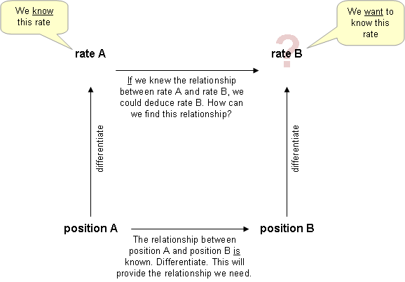
Flow Chart for Related Rate Problem Solving: Related rate problems cab be handled by taking a methodical approach.
Higher Derivatives
The derivative of an already-differentiated expression is called a higher-order derivative.Learning Objectives
Compute higher (second, third, etc.) derivatives of functionsKey Takeaways
Key Points
- The second derivative, or second order derivative, is the derivative of the derivative of a function.
- Because the derivative of a function is defined as a function representing the slope of the original function, the double derivative is the function representing the slope of the first-derivative function.
- If [latex]x(t)[/latex] represents the position of an object at time [latex]t[/latex], then the higher-order derivatives of [latex]x[/latex] have physical interpretations, such as velocity and acceleration.
Key Terms
- derivative: a measure of how a function changes as its input changes
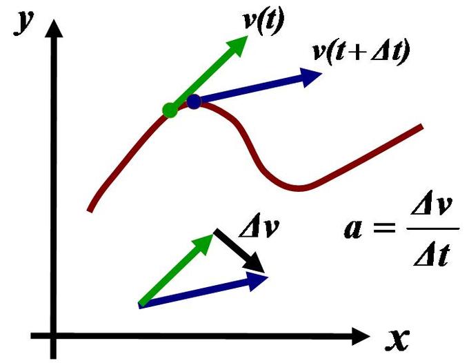
Acceleration: Acceleration is the time-rate of change of velocity, and the second-order rate of change of position.
- [latex]f'(x) = 15x^2 + 6x - 1[/latex]
- [latex]f''(x) = 30x + 6[/latex]
- [latex]f'''(x) = 30[/latex]
Licenses & Attributions
CC licensed content, Shared previously
- Curation and Revision. Provided by: Boundless.com License: CC BY-SA: Attribution-ShareAlike.
CC licensed content, Specific attribution
- Derivative. Provided by: Wikipedia License: CC BY-SA: Attribution-ShareAlike.
- Tangent. Provided by: Wikipedia License: CC BY-SA: Attribution-ShareAlike.
- secant. Provided by: Wiktionary License: CC BY-SA: Attribution-ShareAlike.
- tangent. Provided by: Wiktionary License: CC BY-SA: Attribution-ShareAlike.
- Tangent. Provided by: Wikipedia License: Public Domain: No Known Copyright.
- Calculus/Differentiation/Differentiation Defined. Provided by: Wikibooks License: CC BY-SA: Attribution-ShareAlike.
- Derivative. Provided by: Wikipedia Located at: https://en.wikipedia.org/wiki/Derivative. License: CC BY-SA: Attribution-ShareAlike.
- slope. Provided by: Wiktionary License: CC BY-SA: Attribution-ShareAlike.
- Tangent. Provided by: Wikipedia License: Public Domain: No Known Copyright.
- Derivative. Provided by: Wikipedia License: Public Domain: No Known Copyright.
- Derivative. Provided by: Wikipedia License: CC BY-SA: Attribution-ShareAlike.
- domain. Provided by: Wiktionary License: CC BY-SA: Attribution-ShareAlike.
- range. Provided by: Wiktionary License: CC BY-SA: Attribution-ShareAlike.
- Tangent. Provided by: Wikipedia License: Public Domain: No Known Copyright.
- Derivative. Provided by: Wikipedia License: Public Domain: No Known Copyright.
- Tangent-calculus.png. Provided by: Wikipedia License: CC BY-SA: Attribution-ShareAlike.
- Right-continuous.png. Provided by: Wikipedia License: CC BY-SA: Attribution-ShareAlike.
- Derivative. Provided by: Wikipedia License: CC BY-SA: Attribution-ShareAlike.
- Calculus/Product and Quotient Rules. Provided by: Wikibooks License: CC BY-SA: Attribution-ShareAlike.
- difference quotient. Provided by: Wikipedia License: CC BY-SA: Attribution-ShareAlike.
- polynomial. Provided by: Wiktionary License: CC BY-SA: Attribution-ShareAlike.
- Tangent. Provided by: Wikipedia License: Public Domain: No Known Copyright.
- Derivative. Provided by: Wikipedia License: Public Domain: No Known Copyright.
- Tangent-calculus.png. Provided by: Wikipedia License: CC BY-SA: Attribution-ShareAlike.
- Right-continuous.png. Provided by: Wikipedia License: CC BY-SA: Attribution-ShareAlike.
- Calculus/Product and Quotient Rules. Provided by: Wikibooks License: CC BY-SA: Attribution-ShareAlike.
- Calculus/Derivatives of Trigonometric Functions. Provided by: Wikibooks License: CC BY-SA: Attribution-ShareAlike.
- Trigonometric function. Provided by: Wikipedia License: CC BY-SA: Attribution-ShareAlike.
- secant. Provided by: Wiktionary License: CC BY-SA: Attribution-ShareAlike.
- Tangent. Provided by: Wikipedia License: Public Domain: No Known Copyright.
- Derivative. Provided by: Wikipedia License: Public Domain: No Known Copyright.
- Tangent-calculus.png. Provided by: Wikipedia License: CC BY-SA: Attribution-ShareAlike.
- Right-continuous.png. Provided by: Wikipedia License: CC BY-SA: Attribution-ShareAlike.
- Calculus/Product and Quotient Rules. Provided by: Wikibooks License: CC BY-SA: Attribution-ShareAlike.
- Sine_cosine_one_period.png. Provided by: Wikipedia License: CC BY-SA: Attribution-ShareAlike.
- Chain rule. Provided by: Wikipedia License: CC BY-SA: Attribution-ShareAlike.
- Calculus/Chain Rule. Provided by: Wikibooks License: CC BY-SA: Attribution-ShareAlike.
- composite. Provided by: Wiktionary License: CC BY-SA: Attribution-ShareAlike.
- Tangent. Provided by: Wikipedia License: Public Domain: No Known Copyright.
- Derivative. Provided by: Wikipedia License: Public Domain: No Known Copyright.
- Tangent-calculus.png. Provided by: Wikipedia License: CC BY-SA: Attribution-ShareAlike.
- Right-continuous.png. Provided by: Wikipedia License: CC BY-SA: Attribution-ShareAlike.
- Calculus/Product and Quotient Rules. Provided by: Wikibooks License: CC BY-SA: Attribution-ShareAlike.
- Sine_cosine_one_period.png. Provided by: Wikipedia License: CC BY-SA: Attribution-ShareAlike.
- Skydiving. Provided by: Wikipedia License: CC BY-SA: Attribution-ShareAlike.
- Implicit differentiation. Provided by: Wikipedia License: CC BY-SA: Attribution-ShareAlike.
- implicit. Provided by: Wiktionary License: CC BY-SA: Attribution-ShareAlike.
- Tangent. Provided by: Wikipedia License: Public Domain: No Known Copyright.
- Derivative. Provided by: Wikipedia License: Public Domain: No Known Copyright.
- Tangent-calculus.png. Provided by: Wikipedia License: CC BY-SA: Attribution-ShareAlike.
- Right-continuous.png. Provided by: Wikipedia License: CC BY-SA: Attribution-ShareAlike.
- Calculus/Product and Quotient Rules. Provided by: Wikibooks License: CC BY-SA: Attribution-ShareAlike.
- Sine_cosine_one_period.png. Provided by: Wikipedia License: CC BY-SA: Attribution-ShareAlike.
- Skydiving. Provided by: Wikipedia License: CC BY-SA: Attribution-ShareAlike.
- Implicit function theorem. Provided by: Wikipedia License: CC BY-SA: Attribution-ShareAlike.
- differential geometry. Provided by: Wiktionary License: CC BY-SA: Attribution-ShareAlike.
- Differential calculus. Provided by: Wikipedia License: CC BY-SA: Attribution-ShareAlike.
- momentum. Provided by: Wiktionary License: CC BY-SA: Attribution-ShareAlike.
- gross domestic product. Provided by: Wiktionary License: CC BY-SA: Attribution-ShareAlike.
- Tangent. Provided by: Wikipedia License: Public Domain: No Known Copyright.
- Derivative. Provided by: Wikipedia License: Public Domain: No Known Copyright.
- Tangent-calculus.png. Provided by: Wikipedia License: CC BY-SA: Attribution-ShareAlike.
- Right-continuous.png. Provided by: Wikipedia License: CC BY-SA: Attribution-ShareAlike.
- Calculus/Product and Quotient Rules. Provided by: Wikibooks License: CC BY-SA: Attribution-ShareAlike.
- Sine_cosine_one_period.png. Provided by: Wikipedia License: CC BY-SA: Attribution-ShareAlike.
- Skydiving. Provided by: Wikipedia License: CC BY-SA: Attribution-ShareAlike.
- Implicit function theorem. Provided by: Wikipedia License: CC BY-SA: Attribution-ShareAlike.
- Calculus/Related Rates. Provided by: Wikibooks License: CC BY-SA: Attribution-ShareAlike.
- Related rates. Provided by: Wikipedia License: CC BY-SA: Attribution-ShareAlike.
- variable. Provided by: Wiktionary License: CC BY-SA: Attribution-ShareAlike.
- Tangent. Provided by: Wikipedia License: Public Domain: No Known Copyright.
- Derivative. Provided by: Wikipedia License: Public Domain: No Known Copyright.
- Tangent-calculus.png. Provided by: Wikipedia License: CC BY-SA: Attribution-ShareAlike.
- Right-continuous.png. Provided by: Wikipedia License: CC BY-SA: Attribution-ShareAlike.
- Calculus/Product and Quotient Rules. Provided by: Wikibooks License: CC BY-SA: Attribution-ShareAlike.
- Sine_cosine_one_period.png. Provided by: Wikipedia License: CC BY-SA: Attribution-ShareAlike.
- Skydiving. Provided by: Wikipedia License: CC BY-SA: Attribution-ShareAlike.
- Implicit function theorem. Provided by: Wikipedia License: CC BY-SA: Attribution-ShareAlike.
- Related rates. Provided by: Wikipedia License: Public Domain: No Known Copyright.
- Calculus/Higher Order Derivatives. Provided by: Wikibooks License: CC BY-SA: Attribution-ShareAlike.
- Derivative. Provided by: Wikipedia License: CC BY-SA: Attribution-ShareAlike.
- derivative. Provided by: Wikipedia License: CC BY-SA: Attribution-ShareAlike.
- Tangent. Provided by: Wikipedia Located at: https://en.wikipedia.org/wiki/Tangent. License: Public Domain: No Known Copyright.
- Derivative. Provided by: Wikipedia License: Public Domain: No Known Copyright.
- Tangent-calculus.png. Provided by: Wikipedia License: CC BY-SA: Attribution-ShareAlike.
- Right-continuous.png. Provided by: Wikipedia License: CC BY-SA: Attribution-ShareAlike.
- Calculus/Product and Quotient Rules. Provided by: Wikibooks License: CC BY-SA: Attribution-ShareAlike.
- Sine_cosine_one_period.png. Provided by: Wikipedia License: CC BY-SA: Attribution-ShareAlike.
- Skydiving. Provided by: Wikipedia License: CC BY-SA: Attribution-ShareAlike.
- Implicit function theorem. Provided by: Wikipedia License: CC BY-SA: Attribution-ShareAlike.
- Related rates. Provided by: Wikipedia License: Public Domain: No Known Copyright.
- Acceleration. Provided by: Wikipedia License: CC BY-SA: Attribution-ShareAlike.
