Applications of Differentiation
Linear Approximation
A linear approximation is an approximation of a general function using a linear function.Learning Objectives
Estimate a function's output using linear approximationKey Takeaways
Key Points
- By taking the derivative one may find the slope of a function.
- The values between two points can be approximated as lying on a straight line between those points, where the line is tangent to the function at one of the points.
- Linear approximation can be made arbitrarily accurate by decreasing the distance between the sample points.
Key Terms
- linear: having the form of a line; straight
- differentiable: having a derivative, said of a function whose domain and co-domain are manifolds
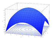
Maximum and Minimum Values
Maxima and minima are critical points on graphs and can be found by the first derivative and the second derivative.Learning Objectives
Use the first and second derivative to find critical points (maxima and minima) on graphs of functionsKey Takeaways
Key Points
- The critical point of a function is a value for which the first derivative of the function is 0, or undefined.
- A critical point often indicates a maximum or a minimum, or the endpoint of an interval.
- If the second derivative at a critical point is positive then it is a minimum, and if it is negative then it is a maximum.
Key Terms
- critical point: a maximum, minimum, or point of inflection on a curve; a point at which the derivative of a function is zero or undefined

Maxima and Minima: Local and global maxima and minima for [latex]\cos \frac{3πx}{x}[/latex], [latex]0.1 \leq x \leq 1.1[/latex].
The Mean Value Theorem, Rolle's Theorem, and Monotonicity
The MVT states that for a function continuous on an interval, the mean value of the function on the interval is a value of the function.Learning Objectives
Use the Mean Value Theorem and Rolle's Theorem to reach conclusions about points on continuous and differentiable functionsKey Takeaways
Key Points
- In calculus, the mean value theorem states, roughly: given a planar arc between two endpoints, there is at least one point at which the tangent to the arc is parallel to the secant through its endpoints.
- More precisely, if a function [latex]f[/latex] is continuous on the closed interval [latex][a, b][/latex], where [latex]a < b[/latex], and differentiable on the open interval [latex](a, b)[/latex], then there exists a point [latex]c[/latex] in [latex](a, b)[/latex] such that [latex]f'(c)=\frac{f(b)-f(a)}{b-a}[/latex].
- Rolle's Theorem states that if a real-valued function [latex]f[/latex] is continuous on a closed interval [latex][a, b][/latex], differentiable on the open interval [latex](a, b)[/latex], and [latex]f(a) = f(b)[/latex], then there exists a point [latex]c[/latex] in the open interval [latex](a, b)[/latex] such that [latex]f'(c)=0[/latex].
Key Terms
- mean: The average value.
- secant: a straight line that intersects a curve at two or more points
- tangent: a straight line touching a curve at a single point without crossing it there

Mean Value Theorem: For any function that is continuous on [latex][a, b][/latex] and differentiable on [latex](a, b)[/latex] there exists some [latex]c[/latex] in the interval [latex](a, b)[/latex] such that the secant joining the endpoints of the interval [latex][a, b][/latex] is parallel to the tangent at [latex]c[/latex].
Derivatives and the Shape of the Graph
The shape of a graph may be found by taking derivatives to tell you the slope and concavity.Learning Objectives
Sketch the shape of a graph by using differentiation to find the slope and concavityKey Takeaways
Key Points
- The derivative of a function is the the function that defines the slope of the graph at each point.
- The second derivative of the graph tells you the concavity of the graph at a point.
- Inflection points are where the second derivative is 0 and are points where the concavity changes.
Key Terms
- concave: curved like the inner surface of a sphere or bowl
- convex: curved or bowed outward like the outside of a bowl or sphere or circle
Inflection Point
A point where the second derivative of a function changes sign is called an inflection point. At an inflection point, the second derivative may be zero, as in the case of the inflection point [latex]x=0[/latex] of the function [latex]y=x^3[/latex], or it may fail to exist, as in the case of the inflection point [latex]x=0[/latex] of the function [latex]y=x^{\frac{1}{3}}[/latex]. At an inflection point, a function switches from being a convex function to being a concave function or vice versa.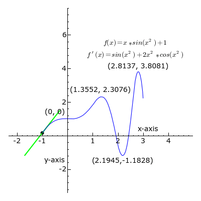
Derivative: At each point, the derivative of is the slope of a line that is tangent to the curve. The line is always tangent to the blue curve; its slope is the derivative. Note derivative is positive where a green line appears, negative where a red line appears, and zero where a black line appears.
Horizontal Asymptotes and Limits at Infinity
The asymptotes are computed using limits and are classified into horizontal, vertical and oblique depending on the orientation.Learning Objectives
Distinguish three types of asymptotes, identifying curves that can and can not have themKey Takeaways
Key Points
- Horizontal asymptotes are horizontal lines that the graph of the function approaches as [latex]x[/latex] tends toward [latex]+ \infty[/latex] or [latex]- \infty[/latex].
- Vertical asymptotes are vertical lines (perpendicular to the [latex]x[/latex]-axis) near which the function grows without bound.
- Oblique asymptotes are diagonal lines so that the difference between the curve and the line approaches [latex]0[/latex] as [latex]x[/latex] tends toward [latex]+ \infty[/latex] or [latex]- \infty[/latex].
Key Terms
- limit: a value to which a sequence or function converges
- arctangent: Any of several single-valued or multivalued functions that are inverses of the tangent function.
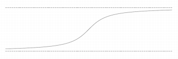
Horizontal asymptote: The graph of a function can have two horizontal asymptotes. An example of such a function would be [latex]y = \arctan(x)[/latex].
Curve Sketching
Curve sketching is used to produce a rough idea of overall shape of a curve given its equation without computing a detailed plot.Learning Objectives
Use "curve sketching" to estimate a function's shapeKey Takeaways
Key Points
- Determine the [latex]x[/latex]- and [latex]y[/latex]-intercepts of the curve.
- Determine the symmetry of the curve.
- Determine any bounds on the values of [latex]x[/latex] and [latex]y[/latex].
- Determine the asymptotes of the curve.
Key Terms
- symmetry: Exact correspondence on either side of a dividing line, plane, center or axis.
- asymptote: a straight line which a curve approaches arbitrarily closely, as they go to infinity
- Determine the [latex]x[/latex]- and [latex]y[/latex]-intercepts of the curve. The [latex]x[/latex]-intercepts are found by setting [latex]y[/latex] equal to [latex]0[/latex] in the equation of the curve and solving for [latex]x[/latex]. Similarly, the y intercepts are found by setting [latex]x[/latex] equal to [latex]0[/latex] in the equation of the curve and solving for [latex]y[/latex].
- Determine the symmetry of the curve. If the exponent of [latex]x[/latex] is always even in the equation of the curve, then the [latex]y[/latex]- axis is an axis of symmetry for the curve. Similarly, if the exponent of [latex]y[/latex] is always even in the equation of the curve, then the [latex]x[/latex]-axis is an axis of symmetry for the curve. If the sum of the degrees of [latex]x[/latex] and [latex]y[/latex] in each term is always even or always odd, then the curve is symmetric about the origin and the origin is called a center of the curve.
- Determine any bounds on the values of [latex]x[/latex] and [latex]y[/latex]. If the curve passes through the origin then determine the tangent lines there. For algebraic curves, this can be done by removing all but the terms of lowest order from the equation and solving. Similarly, removing all but the terms of highest order from the equation and solving gives the points where the curve meets the line at infinity.
- Determine the asymptotes of the curve. Also determine from which side the curve approaches the asymptotes and where the asymptotes intersect the curve.
Graphing on Computers and Calculators
Graphics can be created by hand, using computer programs, and with graphing calculators.Learning Objectives
Demonstrate how computers and calculators can speed up and simplify graphingKey Takeaways
Key Points
- A graphing calculator is a handheld scientific calculator capable of plotting graphs, solving simultaneous equations, and performing numerous other tasks with variables.
- Graphs can be created using open source and proprietary computer programs.
- High end features of computer programs include speed, high-resolution, and tree-dimensional graphing.
Key Terms
- proprietary: Manufactured exclusively by the owner of intellectual property rights (IPR), as with a patent or trade secret.
- scientific calculator: An electronic calculator that can handle trigonometric, exponential and often other advanced functions, and can show its output in scientific notation and sometimes in hexadecimal, octal or binary
- graph: A diagram displaying data; in particular one showing the relationship between two or more quantities, measurements or indicative numbers that may or may not have a specific mathematical formula relating them to each other.
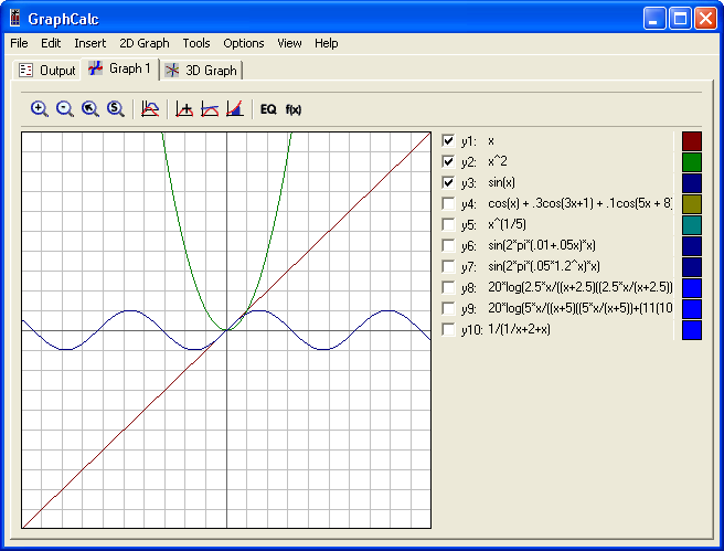
GraphCalc: Screenshot of GraphCalc
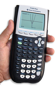
Graphing Calculator: Calculators graph curves by drawing each pixel as a linear approximation of the function.
Optimization
Mathematical optimization is the selection of a best element (with regard to some criteria) from some set of available alternatives.Learning Objectives
Define optimization as finding the maxima and minima for a function, and describe its real-life applicationsKey Takeaways
Key Points
- Many design problems can also be expressed as optimization programs.
- Optimization relies heavily on finding maxima and minima. For this, calculus is useful.
- An example would be companies seeking to maximize sales while minimizing costs.
Key Terms
- optimization: the design and operation of a system or process to make it as good as possible in some defined sense
- stochastic: Random, randomly determined
Maxima: Finding maxima is useful in optimization problems.
Newton's Method
Newton's Method is a method for finding successively better approximations to the roots (or zeroes) of a real-valued function.Learning Objectives
Use "Newton's Method" to find successively more accurate estimates for a function's [latex]x[/latex]-interceptKey Takeaways
Key Points
- Newton's method proceeds by an initial guess which is reasonably close to the true root, then the function is approximated by its tangent line (which can be computed using the tools of calculus).
- Then compute the [latex]x[/latex]-intercept of this tangent line (which is easily done with elementary algebra). This [latex]x[/latex]-intercept will typically be a better approximation to the function's root than the original guess, and the method can be iterated.
- The more times you iterate, the more accurate the approximation to the actual roots.
Key Terms
- derivative: a measure of how a function changes as its input changes
- root: A zero (of a function).
- tangent: a straight line touching a curve at a single point without crossing it there
- Given a function ƒ defined over the reals x, and its derivative ƒ ', we begin with a first guess x0 for a root of the function f. Provided the function satisfies all the assumptions made in the derivation of the formula, a better approximation x1 is x0 - f(x0) / f'(x0). Geometrically, (x1, 0) is the intersection with the x-axis of a line tangent to f at (x0, f (x0)).The process is repeated as xn+1 = xn - f(xn / f'(xn) until a sufficiently accurate value is reached.
Newton's Method: The function [latex]f[/latex] is shown in blue and the tangent line in red. We see that [latex]x_{n+1}[/latex] is a better approximation than [latex]x_n[/latex] for the root [latex]x[/latex] of the function [latex]f[/latex].
Concavity and the Second Derivative Test
The second derivative test is a criterion for determining whether a given critical point is a local maximum or a local minimum.Learning Objectives
Calculate whether a function has a local maximum or minimum at a critical point using the second derivative testKey Takeaways
Key Points
- A critical point is a point where the derivative is 0.
- If the second derivative is positive, the point is a minimum.
- If the second derivative is negative, the point is a maximum.
- If the second derivative is 0, the test is inconclusive.
Key Terms
- local minimum: A point on a graph (or its associated function) such that the points each side have a greater value even though another point exists with a smaller value.
- local maximum: A maximum within a restricted domain, especially a point on a function whose value is greater than the values of all other points near it.
- critical point: a maximum, minimum, or point of inflection on a curve; a point at which the derivative of a function is zero or undefined
Maxima and Minima: Telling whether a critical point is a maximum or a minimum has to do with the second derivative. If it is concave-up at the point, it is a minimum; if concave-down, it is a maximum.
Proof of the Second Derivative Test:
Suppose we have [latex]f''(x) > 0[/latex] (the proof for [latex]f''(x) < 0[/latex] is analogous). By assumption, [latex]f'(x) = 0[/latex]. Then, [latex-display]\displaystyle{0 < f''(x) = \lim_{h \to 0} \frac{f'(x+h)-f'(x)}{h}}[/latex-display] Thus, for a sufficiently small [latex]h[/latex] we get [latex-display]\displaystyle{\frac{f'(x+h)}{h} > 0}[/latex-display] which means that [latex]f'(x+h) < 0[/latex] if [latex]h < 0[/latex] (intuitively, [latex]f[/latex] is decreasing as it approaches [latex]x[/latex] from the left), and that [latex]f'(x+h) > 0[/latex] if [latex]h > 0[/latex] (intuitively, [latex]f[/latex] is increasing as we go right from [latex]x[/latex]). Now, by the first derivative test, [latex]f(x)[/latex] has a local minimum at [latex]x[/latex]. A related but distinct use of second derivatives is to determine whether a function is concave up or concave down at a point. It does not, however, provide information about inflection points. Specifically, a twice-differentiable function [latex]f[/latex] is concave-up if [latex]f''(x)[/latex] is positive and concave-down if [latex]f''(x)[/latex] is negative.Differentials
Differentials are the principal part of the change in a function [latex]y = f(x)[/latex] with respect to changes in the independent variable.Learning Objectives
Use implicit differentiation to find the derivatives of functions that are not explicitly functions of [latex]x[/latex]Key Takeaways
Key Points
- Differentials are notated by [latex]dx[/latex] or [latex]dy[/latex].
- They represent an infinitesimal increase in the variable [latex]x[/latex] or [latex]y[/latex].
- Higher order differentials represent successive derivatives.
Key Terms
- infinitesimal: a non-zero quantity whose magnitude is smaller than any positive number
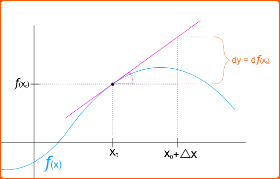
Differentials: The differential of a function [latex]f(x)[/latex] at a point [latex]x_0[/latex].
Licenses & Attributions
CC licensed content, Shared previously
- Curation and Revision. Provided by: Boundless.com License: CC BY-SA: Attribution-ShareAlike.
CC licensed content, Specific attribution
- Linear approximation. Provided by: Wikipedia License: CC BY-SA: Attribution-ShareAlike.
- linear. Provided by: Wiktionary License: CC BY-SA: Attribution-ShareAlike.
- differentiable. Provided by: Wiktionary License: CC BY-SA: Attribution-ShareAlike.
- critical point. Provided by: Wiktionary Located at: https://en.wiktionary.org/wiki/critical_point. License: CC BY-SA: Attribution-ShareAlike.
- Maxima and minima. Provided by: Wikipedia License: CC BY-SA: Attribution-ShareAlike.
- Maxima and minima. Provided by: Wikipedia License: CC BY: Attribution.
- Rolle's theorem. Provided by: Wikipedia License: CC BY-SA: Attribution-ShareAlike.
- Mean value theorem. Provided by: Wikipedia License: CC BY-SA: Attribution-ShareAlike.
- Boundless. Provided by: Boundless Learning License: CC BY-SA: Attribution-ShareAlike.
- tangent. Provided by: Wiktionary Located at: https://en.wiktionary.org/wiki/tangent. License: CC BY-SA: Attribution-ShareAlike.
- secant. Provided by: Wiktionary License: CC BY-SA: Attribution-ShareAlike.
- Maxima and minima. Provided by: Wikipedia License: CC BY: Attribution.
- Mean value theorem. Provided by: Wikipedia License: CC BY: Attribution.
- Derivative. Provided by: Wikipedia License: CC BY-SA: Attribution-ShareAlike.
- Derivative. Provided by: Wikipedia License: CC BY-SA: Attribution-ShareAlike.
- Boundless. Provided by: Boundless Learning License: CC BY-SA: Attribution-ShareAlike.
- convex. Provided by: Wiktionary License: CC BY-SA: Attribution-ShareAlike.
- Maxima and minima. Provided by: Wikipedia License: CC BY: Attribution.
- Mean value theorem. Provided by: Wikipedia License: CC BY: Attribution.
- Derivative. Provided by: Wikipedia License: CC BY: Attribution.
- Asymptote. Provided by: Wikipedia License: CC BY-SA: Attribution-ShareAlike.
- arctangent. Provided by: Wiktionary License: CC BY-SA: Attribution-ShareAlike.
- limit. Provided by: Wiktionary License: CC BY-SA: Attribution-ShareAlike.
- Maxima and minima. Provided by: Wikipedia Located at: https://en.wikipedia.org/wiki/Maxima_and_minima. License: CC BY: Attribution.
- Mean value theorem. Provided by: Wikipedia License: CC BY: Attribution.
- Derivative. Provided by: Wikipedia License: CC BY: Attribution.
- Asymptote. Provided by: Wikipedia License: CC BY: Attribution.
- Curve sketching. Provided by: Wikipedia License: CC BY-SA: Attribution-ShareAlike.
- symmetry. Provided by: Wiktionary License: CC BY-SA: Attribution-ShareAlike.
- asymptote. Provided by: Wiktionary License: CC BY-SA: Attribution-ShareAlike.
- Maxima and minima. Provided by: Wikipedia License: CC BY: Attribution.
- Mean value theorem. Provided by: Wikipedia License: CC BY: Attribution.
- Derivative. Provided by: Wikipedia License: CC BY: Attribution.
- Asymptote. Provided by: Wikipedia License: CC BY: Attribution.
- GraphCalc. Provided by: Wikipedia License: CC BY-SA: Attribution-ShareAlike.
- Mathematica. Provided by: Wikipedia License: CC BY-SA: Attribution-ShareAlike.
- Information graphics. Provided by: Wikipedia License: CC BY-SA: Attribution-ShareAlike.
- Graphing calculator. Provided by: Wikipedia License: CC BY-SA: Attribution-ShareAlike.
- proprietary. Provided by: Wiktionary License: CC BY-SA: Attribution-ShareAlike.
- graph. Provided by: Wiktionary License: CC BY-SA: Attribution-ShareAlike.
- scientific calculator. Provided by: Wiktionary License: CC BY-SA: Attribution-ShareAlike.
- Maxima and minima. Provided by: Wikipedia License: CC BY: Attribution.
- Mean value theorem. Provided by: Wikipedia License: CC BY: Attribution.
- Derivative. Provided by: Wikipedia License: CC BY: Attribution.
- Asymptote. Provided by: Wikipedia License: CC BY: Attribution.
- Graphing calculator. Provided by: Wikipedia License: CC BY: Attribution.
- Provided by: Wikimedia Located at: https://upload.wikimedia.org/wikipedia/commons/d/d9/Graphcalc_screenshot.png. License: CC BY-SA: Attribution-ShareAlike.
- Mathematical optimization. Provided by: Wikipedia License: CC BY-SA: Attribution-ShareAlike.
- Karushu2013Kuhnu2013Tucker conditions. Provided by: Wikipedia License: CC BY-SA: Attribution-ShareAlike.
- Mathematical optimization. Provided by: Wikipedia License: CC BY-SA: Attribution-ShareAlike.
- optimization. Provided by: Wiktionary License: CC BY-SA: Attribution-ShareAlike.
- stochastic. Provided by: Wiktionary License: CC BY-SA: Attribution-ShareAlike.
- Maxima and minima. Provided by: Wikipedia License: CC BY: Attribution.
- Mean value theorem. Provided by: Wikipedia License: CC BY: Attribution.
- Derivative. Provided by: Wikipedia License: CC BY: Attribution.
- Asymptote. Provided by: Wikipedia License: CC BY: Attribution.
- Graphing calculator. Provided by: Wikipedia Located at: https://en.wikipedia.org/wiki/Graphing_calculator. License: CC BY: Attribution.
- Provided by: Wikimedia Located at: https://upload.wikimedia.org/wikipedia/commons/d/d9/Graphcalc_screenshot.png. License: CC BY-SA: Attribution-ShareAlike.
- Mathematical optimization. Provided by: Wikipedia License: CC BY: Attribution.
- Newton's method. Provided by: Wikipedia License: CC BY-SA: Attribution-ShareAlike.
- derivative. Provided by: Wikipedia License: CC BY-SA: Attribution-ShareAlike.
- tangent. Provided by: Wiktionary License: CC BY-SA: Attribution-ShareAlike.
- root. Provided by: Wiktionary License: CC BY-SA: Attribution-ShareAlike.
- Maxima and minima. Provided by: Wikipedia License: CC BY: Attribution.
- Mean value theorem. Provided by: Wikipedia License: CC BY: Attribution.
- Derivative. Provided by: Wikipedia License: CC BY: Attribution.
- Asymptote. Provided by: Wikipedia License: CC BY: Attribution.
- Graphing calculator. Provided by: Wikipedia License: CC BY: Attribution.
- Provided by: Wikimedia Located at: https://upload.wikimedia.org/wikipedia/commons/d/d9/Graphcalc_screenshot.png. License: CC BY-SA: Attribution-ShareAlike.
- Mathematical optimization. Provided by: Wikipedia License: CC BY: Attribution.
- Newton's method. Provided by: Wikipedia License: CC BY: Attribution.
- Second derivative test. Provided by: Wikipedia License: CC BY-SA: Attribution-ShareAlike.
- critical point. Provided by: Wiktionary License: CC BY-SA: Attribution-ShareAlike.
- local maximum. Provided by: Wiktionary License: CC BY-SA: Attribution-ShareAlike.
- local minimum. Provided by: Wiktionary License: CC BY-SA: Attribution-ShareAlike.
- Maxima and minima. Provided by: Wikipedia License: CC BY: Attribution.
- Mean value theorem. Provided by: Wikipedia License: CC BY: Attribution.
- Derivative. Provided by: Wikipedia License: CC BY: Attribution.
- Asymptote. Provided by: Wikipedia License: CC BY: Attribution.
- Graphing calculator. Provided by: Wikipedia License: CC BY: Attribution.
- Provided by: Wikimedia Located at: https://upload.wikimedia.org/wikipedia/commons/d/d9/Graphcalc_screenshot.png. License: CC BY-SA: Attribution-ShareAlike.
- Mathematical optimization. Provided by: Wikipedia License: CC BY: Attribution.
- Newton's method. Provided by: Wikipedia License: CC BY: Attribution.
- Maxima and minima. Provided by: Wikipedia License: CC BY: Attribution.
- Differential of a function. Provided by: Wikipedia License: CC BY-SA: Attribution-ShareAlike.
- infinitesimal. Provided by: Wiktionary License: CC BY-SA: Attribution-ShareAlike.
- Maxima and minima. Provided by: Wikipedia License: CC BY: Attribution.
- Mean value theorem. Provided by: Wikipedia License: CC BY: Attribution.
- Derivative. Provided by: Wikipedia License: CC BY: Attribution.
- Asymptote. Provided by: Wikipedia License: CC BY: Attribution.
- Graphing calculator. Provided by: Wikipedia License: CC BY: Attribution.
- Provided by: Wikimedia Located at: https://upload.wikimedia.org/wikipedia/commons/d/d9/Graphcalc_screenshot.png. License: CC BY-SA: Attribution-ShareAlike.
- Mathematical optimization. Provided by: Wikipedia Located at: https://en.wikipedia.org/wiki/Mathematical_optimization. License: CC BY: Attribution.
- Newton's method. Provided by: Wikipedia License: CC BY: Attribution.
- Maxima and minima. Provided by: Wikipedia License: CC BY: Attribution.
- Differentials. Provided by: Wikipedia License: CC BY: Attribution.
