Sequences and Series
Introduction to Sequences
A mathematical sequence is an ordered list of objects, often numbers. Sometimes the numbers in a sequence are defined in terms of a previous number in the list.Learning Objectives
Differentiate between different types of sequencesKey Takeaways
Key Points
- The number of ordered elements (possibly infinite ) is called the length of the sequence. Unlike a set, order matters, and a particular term can appear multiple times at different positions in the sequence.
- An arithmetic sequence is one in which a term is obtained by adding a constant to a previous term of a sequence. So the [latex]n[/latex]th term can be described by the formula [latex]a_n = a_{n-1} + d [/latex].
- A geometric sequence is one in which a term of a sequence is obtained by multiplying the previous term by a constant. It can be described by the formula [latex]a_n=r \cdot a_{n-1}[/latex].
Key Terms
- sequence: An ordered list of elements, possibly infinite in length.
- finite: Limited, constrained by bounds.
- set: A collection of zero or more objects, possibly infinite in size, and disregarding any order or repetition of the objects that may be contained within it.
Sequences
In mathematics, a sequence is an ordered list of objects. Like a set, it contains members (also called elements or terms). The number of ordered elements (possibly infinite) is called the length of the sequence. Unlike a set, order matters, and a particular term can appear multiple times at different positions in the sequence. For example, [latex](M, A, R, Y)[/latex] is a sequence of letters that differs from [latex](A, R, M, Y)[/latex], as the ordering matters, and [latex](1, 1, 2, 3, 5, 8)[/latex], which contains the number 1 at two different positions, is a valid sequence. Sequences can be finite, as in this example, or infinite, such as the sequence of all even positive integers [latex](2, 4, 6, \cdots )[/latex]. Finite sequences are sometimes known as strings or words and infinite sequences as streams.Examples and Notation
Finite and Infinite Sequences
A more formal definition of a finite sequence with terms in a set [latex]S[/latex] is a function from [latex]\left \{ 1, 2, \cdots, n \right \}[/latex] to [latex]S[/latex] for some [latex]n > 0[/latex]. An infinite sequence in [latex]S[/latex] is a function from [latex]\left \{ 1, 2, \cdots \right \}[/latex] to [latex]S[/latex]. For example, the sequence of prime numbers [latex](2,3,5,7,11, \cdots )[/latex] is the function [latex-display]1\rightarrow 2, 2\rightarrow 3, 3\rightarrow 5, 4\rightarrow 7, 5\rightarrow 11, \cdots[/latex-display] A sequence of a finite length n is also called an [latex]n[/latex]-tuple. Finite sequences include the empty sequence [latex]( \quad )[/latex] that has no elements.Recursive Sequences
Many of the sequences you will encounter in a mathematics course are produced by a formula, where some operation(s) is performed on the previous member of the sequence [latex]a_{n-1}[/latex] to give the next member of the sequence [latex]a_n[/latex]. These are called recursive sequences.Arithmetic Sequences
An arithmetic (or linear) sequence is a sequence of numbers in which each new term is calculated by adding a constant value to the previous term. An example is [latex](10,13,16,19,22,25)[/latex]. In this example, the first term (which we will call [latex]a_1[/latex]) is [latex]10[/latex], and the common difference ([latex]d[/latex])—that is, the difference between any two adjacent numbers—is [latex]3[/latex]. The recursive definition is therefore [latex-display]\displaystyle{a_n=a_{n-1}+3, a_1=10}[/latex-display] Another example is [latex](25,22,19,16,13,10)[/latex]. In this example [latex]a_1 = 25[/latex], and [latex]d=-3[/latex]. The recursive definition is therefore [latex-display]\displaystyle{a_n=a_{n-1}-3, a_1=25}[/latex-display] In both of these examples, [latex]n[/latex] (the number of terms) is [latex]6[/latex].Geometric Sequences
A geometric sequence is a list in which each number is generated by multiplying a constant by the previous number. An example is [latex](2,6,18,54,162)[/latex]. In this example, [latex]a_1=2[/latex], and the common ratio ([latex]r[/latex])—that is, the ratio between any two adjacent numbers—is 3. Therefore the recursive definition is [latex-display]a_n=3a_{n-1}, a_1=2[/latex-display] Another example is [latex](162,54,18,6,2)[/latex]. In this example [latex]a_1=162[/latex], and [latex]\displaystyle{r=\frac{1}{3}}[/latex]. Therefore the recursive formula is [latex-display]\displaystyle{a_n=\frac13\cdot a_{n-1}, a_1=162}[/latex-display] In both examples [latex]n=5[/latex].Explicit Definitions
An explicit definition of an arithmetic sequence is one in which the [latex]n[/latex]th term is defined without making reference to the previous term. This is more useful, because it means you can find (for instance) the 20th term without finding all of the other terms in between. To find the explicit definition of an arithmetic sequence, you begin writing out the terms. Assume our sequence is [latex]t_1, t_2, \dots [/latex]. The first term is always [latex]t_1[/latex]. The second term goes up by [latex]d[/latex], and so it is [latex]t_1+d[/latex]. The third term goes up by [latex]d[/latex] again, and so it is [latex](t_1+d)+d,[/latex] or in other words, [latex]t_1+2d[/latex]. So we see that: [latex]\displaystyle{ \begin{align} t_1 &= t_1 \\ t_2 &= t_1+d \\ t_3 &= t_1+2d \\ t_4 &= t_1+3d \\ &\vdots \end{align} }[/latex] and so on. From this you can see the generalization that: [latex-display]t_n = t_1+(n-1)d[/latex-display] which is the explicit definition we were looking for. The explicit definition of a geometric sequence is obtained in a similar way. The first term is [latex]t_1[/latex]; the second term is [latex]r[/latex] times that, or [latex]t_1r[/latex]; the third term is [latex]r[/latex] times that, or [latex]t_1r^2[/latex]; and so on. So the general rule is: [latex-display]t_n=t_1 \cdot r^{n-1}[/latex-display]The General Term of a Sequence
Given terms in a sequence, it is often possible to find a formula for the general term of the sequence, if the formula is a polynomial.Learning Objectives
Practice finding a formula for the general term of a sequenceKey Takeaways
Key Points
- Given terms in a sequence generated by a polynomial, there is a method to determine the formula for the polynomial.
- By hand, one can take the differences between each term, then the differences between the differences in terms, etc. If the differences eventually become constant, then the sequence is generated by a polynomial formula.
- Once a constant difference is achieved, one can solve equations to generate the formula for the polynomial.
Key Terms
- sequence: A set of things next to each other in a set order; a series
- general term: A mathematical expression containing variables and constants that, when substituting integer values for each variable, produces a valid term in a sequence.
Linear Polynomials
Consider the sequence: [latex-display]5, 7, 9, 11, 13, \dots[/latex-display] The difference between [latex]7[/latex] and [latex]5[/latex] is [latex]2[/latex]. The difference between [latex]7[/latex] and [latex]9[/latex] is also [latex]2[/latex]. In fact, the difference between each pair of terms is [latex]2[/latex]. Since this difference is constant, and this is the first set of differences, the sequence is given by a first-degree (linear) polynomial. Suppose the formula for the sequence is given by [latex]an+b[/latex] for some constants [latex]a[/latex] and [latex]b[/latex]. Then the sequence looks like: [latex-display]a+b, 2a+b, 3a+b, \dots[/latex-display] The difference between each term and the term after it is [latex]a[/latex]. In our example, [latex]a=2[/latex]. It is possible to solve for [latex]b[/latex] using one of the terms in the sequence. Using the first number in the sequence and the first term: [latex]\displaystyle{ \begin{align} 5 &= a+b \\ b &= 5-a \\ b &= 5-(2)\\ b &= 3 \end{align} }[/latex] So, the [latex]n[/latex]th term of the sequence is given by [latex]2n+3[/latex].Quadratic Polynomials
Suppose the [latex]n[/latex]th term of a sequence was given by [latex]an^2+bn+c[/latex]. Then the sequence would look like: [latex-display]a+b+c, 4a+2b+c, 9a+3b+c, \dots[/latex-display] This sequence was created by plugging in [latex]1[/latex] for [latex]n[/latex], [latex]2[/latex] for [latex]n[/latex], [latex]3[/latex] for [latex]n[/latex], etc. If we start at the second term, and subtract the previous term from each term in the sequence, we can get a new sequence made up of the differences between terms. The first sequence of differences would be: [latex-display]3a+b, 5a+b, 7a+b, \dots[/latex-display] Now, we take the differences between terms in the new sequence. The second sequence of differences is: [latex-display]2a, 2a, 2a, 2a, \dots[/latex-display] The computed differences have converged to a constant after the second sequence of differences. This means that it was a second-order (quadratic) sequence. Working backward from this, we could find the general term for any quadratic sequence.Example
Consider the sequence: [latex-display]4, -7, -26, -53, -88, -131, \dots[/latex-display] The difference between [latex]-7[/latex] and [latex]4[/latex] is [latex]-11[/latex], and the difference between [latex]-26[/latex] and [latex]-7[/latex] is [latex]-19[/latex]. Finding all these differences, we get a new sequence: [latex-display]-11, -19, -27, -35, -43, \dots[/latex-display] This list is still not constant. However, finding the difference between terms once more, we get: [latex-display]-8, -8, -8, -8, \dots[/latex-display] This fact tells us that there is a polynomial formula describing our sequence. Since we had to do differences twice, it is a second-degree (quadratic) polynomial. We can find the formula by realizing that the constant term is [latex]-8[/latex], and that it can also be expressed by [latex]2a[/latex]. Therefore [latex]a=-4[/latex]. Next we note that the first item in our first list of differences is [latex]-11[/latex], but that generically it is supposed to be [latex]3a+b[/latex], so we must have [latex]3(-4)+b=-11[/latex], and [latex]b=1[/latex]. Finally, note that the first term in the sequence is [latex]4[/latex], and can also be expressed by [latex-display]a+b+c = -4+1+c[/latex-display] So, [latex]c=7[/latex], and the formula that generates the sequence is [latex]-4a^2+b+7c[/latex].General Polynomial Sequences
This method of finding differences can be extended to find the general term of a polynomial sequence of any order. For higher orders, it will take more rounds of taking differences for the differences to become constant, and more back-substitution will be necessary in order to solve for the general term.General Terms of Non-Polynomial Sequences
Some sequences are generated by a general term which is not a polynomial. For example, the geometric sequence [latex]2, 4, 8, 16,\dots[/latex] is given by the general term [latex]2^n[/latex]. Because this term is not a polynomial, taking differences will never result in a constant difference. General terms of non-polynomial sequences can be found by observation, as above, or by other means which are beyond our scope for now. Given any general term, the sequence can be generated by plugging in successive values of [latex]n[/latex].Series and Sigma Notation
Sigma notation, denoted by the uppercase Greek letter sigma [latex]\left ( \Sigma \right ),[/latex] is used to represent summations—a series of numbers to be added together.Learning Objectives
Calculate the sum of a series represented in sigma notationKey Takeaways
Key Points
- A series is a summation performed on a list of numbers. Each term is added to the next, resulting in a sum of all terms.
- Sigma notation is used to represent the summation of a series. In this form, the capital Greek letter sigma [latex]\left ( \Sigma \right )[/latex] is used. The range of terms in the summation is represented in numbers below and above the [latex]\Sigma[/latex] symbol, called indices. The lowest index is written below the symbol and the largest index is written above.
Key Terms
- summation: A series of items to be summed or added.
- sigma: The symbol [latex]\Sigma[/latex], used to indicate summation of a set or series.
Sigma Notation
One way to compactly represent a series is with sigma notation, or summation notation, which looks like this: [latex-display]\displaystyle{\sum _{n=3}^{7}{n^2}}[/latex-display] The main symbol seen is the uppercase Greek letter sigma. It indicates a series. To "unpack" this notation, [latex]n=3[/latex] represents the number at which to start counting ([latex]3[/latex]), and the [latex]7[/latex] represents the point at which to stop. For each term, plug that value of [latex]n[/latex] into the given formula ([latex]n^2[/latex]). This particular formula, which we can read as "the sum as [latex]n[/latex] goes from [latex]3[/latex] to [latex]7[/latex] of [latex]n^2[/latex]," means: [latex-display]\displaystyle{3^2 + 4^2 + 5^2 + 6^2 + 7^2}[/latex-display] More generally, sigma notation can be defined as: [latex-display]\displaystyle{\sum _{ i=m }^{ n }{ x_i }=x_m+x_{m+1}+x_{m+2}+...+x_{n-1}+x_n}[/latex-display] In this formula, i represents the index of summation, [latex]x_i[/latex] is an indexed variable representing each successive term in the series, [latex]m[/latex] is the lower bound of summation, and [latex]n[/latex] is the upper bound of summation. The "[latex]i = m[/latex]" under the summation symbol means that the index [latex]i[/latex] starts out equal to [latex]m[/latex]. The index, [latex]i[/latex], is incremented by [latex]1[/latex] for each successive term, stopping when [latex]i=n[/latex]. Another example is: [latex]\displaystyle{ \begin{align} \sum_{i=3}^6 (i^2+1) &= (3^2+1)+(4^2+1)+(5^2+1)+(6^2+1) \\ &=10+17+26+37 \\ &=90 \end{align} }[/latex] This series sums to [latex]90.[/latex] So we could write: [latex-display]\displaystyle \sum_{i=3}^6 (i^2+1)=90[/latex-display]Other Forms of Sigma Notation
Informal writing sometimes omits the definition of the index and bounds of summation when these are clear from context. For example: [latex-display]\displaystyle{\sum x_i^2=\sum _{ i=1 }^n x_i^2}[/latex-display]Recursive Definitions
A recursive definition of a function defines its values for some inputs in terms of the values of the same function for other inputs.Learning Objectives
Use a recursive formula to find specific terms of a sequenceKey Takeaways
Key Points
- In mathematical logic and computer science, a recursive definition, or inductive definition, is used to define an object in terms of itself.
- The recursive definition for an arithmetic sequence is: [latex]a_n=a_{n-1}+d[/latex]. The recursive definition for a geometric sequence is: [latex]a_n=r \cdot a_{n-1}[/latex].
Recursion
In mathematical logic and computer science, a recursive definition, or inductive definition, is used to define an object in terms of itself. A recursive definition of a function defines values of the function for some inputs in terms of the values of the same function for other inputs. For example, the factorial function [latex]n![/latex] is defined by the rules: [latex-display]0!=1[/latex-display] [latex-display](n+1)!=(n+1)n![/latex-display] This definition is valid because, for all [latex]n[/latex], the recursion eventually reaches the base case of [latex]0[/latex]. For example, we can compute [latex]5![/latex] by realizing that [latex]5!=5\cdot 4![/latex], and that [latex]4!=4\cdot 3![/latex], and that [latex]3!=3\cdot 2![/latex], and that [latex]2!=2\cdot 1!,[/latex] and that: [latex]\displaystyle{ \begin{align} 1! &=1\cdot 0! \\ &= 1\cdot 1 \\ &=1 \end{align} }[/latex] Putting this all together we get: [latex]\displaystyle{ \begin{align} 5! &=5\cdot 4\cdot 3\cdot 2 \cdot 1 \\ &= 120 \end{align} }[/latex]Recursive Formulas for Sequences
When discussing arithmetic sequences, you may have noticed that the difference between two consecutive terms in the sequence could be written in a general way: [latex-display]a_n=a_{n-1}+d[/latex-display] The above equation is an example of a recursive equation since the [latex]n[/latex]th term can only be calculated by considering the previous term in the sequence. Compare this with the equation: [latex-display]a_n=a_1+d(n-1).[/latex-display] In this equation, one can directly calculate the nth-term of the arithmetic sequence without knowing the previous terms. Depending on how the sequence is being used, either the recursive definition or the non-recursive one might be more useful. A recursive geometric sequence follows the formula: [latex-display]a_n=r\cdot a_{n-1}[/latex-display] An applied example of a geometric sequence involves the spread of the flu virus. Suppose each infected person will infect two more people, such that the terms follow a geometric sequence.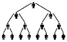 The flu virus is a geometric sequence: Each person infects two more people with the flu virus, making the number of recently-infected people the nth term in a geometric sequence.
Using this equation, the recursive equation for this geometric sequence is:
[latex-display]a_n=2 \cdot a_{n-1}[/latex-display] Recursive equations are extremely powerful. One can work out every term in the series just by knowing previous terms. As can be seen from the examples above, working out and using the previous term [latex]a_{n−1}[/latex] can be a much simpler computation than working out [latex]a_{n}[/latex] from scratch using a general formula. This means that using a recursive formula when using a computer to manipulate a sequence might mean that the calculation will be finished quickly.Licenses & Attributions
CC licensed content, Shared previously
- Curation and Revision. Authored by: Boundless.com. License: Public Domain: No Known Copyright.
CC licensed content, Specific attribution
- Kenny Felder, Advanced Algebra II: Conceptual Explanations. September 17, 2013. Provided by: OpenStax CNX Located at: https://cnx.org/contents/[email protected]:a21bd0c8-710b-4fb6-8bed-66a5afe4610e. License: CC BY: Attribution.
- Free High School Science Texts Project, Sequences and series: Arithmetic & Geometric Sequences, Recursive Formulae (Grade 12). September 17, 2013. Provided by: OpenStax CNX License: CC BY: Attribution.
- Sequence. Provided by: Wikipedia Located at: https://en.wikipedia.org/wiki/Sequence. License: CC BY-SA: Attribution-ShareAlike.
- set. Provided by: Wiktionary License: CC BY-SA: Attribution-ShareAlike.
- finite. Provided by: Wiktionary License: CC BY-SA: Attribution-ShareAlike.
- sequence. Provided by: Wiktionary License: CC BY-SA: Attribution-ShareAlike.
- Sequence. Provided by: Wikipedia License: CC BY-SA: Attribution-ShareAlike.
- Series (mathematics). Provided by: Wikipedia License: CC BY-SA: Attribution-ShareAlike.
- Boundless. Provided by: Boundless Learning License: CC BY-SA: Attribution-ShareAlike.
- sequence. Provided by: Wiktionary License: CC BY-SA: Attribution-ShareAlike.
- series. Provided by: Wiktionary License: CC BY-SA: Attribution-ShareAlike.
- Kenny Felder, Advanced Algebra II: Conceptual Explanations. September 17, 2013. Provided by: OpenStax CNX Located at: https://cnx.org/contents/[email protected]:5063374a-d266-4fb2-acde-454cce78c47c. License: CC BY: Attribution.
- Summation. Provided by: Wikipedia License: CC BY-SA: Attribution-ShareAlike.
- summation. Provided by: Wiktionary License: CC BY-SA: Attribution-ShareAlike.
- vector. Provided by: Wiktionary License: CC BY-SA: Attribution-ShareAlike.
- sigma. Provided by: Wiktionary License: CC BY-SA: Attribution-ShareAlike.
- Free High School Science Texts Project, Sequences and series: Arithmetic & Geometric Sequences, Recursive Formulae (Grade 12). September 17, 2013. Provided by: OpenStax CNX Located at: https://cnx.org/contents/5861a862-139c-4ce9-90ae-3c1f3936728e@1. License: CC BY: Attribution.
- Recursive definition. Provided by: Wikipedia License: CC BY-SA: Attribution-ShareAlike.
- Free High School Science Texts Project, Sequences and Series: Arithmetic & Geometric Sequences, Recursive Formulae (Grade 12). December 10, 2012. Provided by: OpenStax CNX Located at: https://cnx.org/contents/5861a862-139c-4ce9-90ae-3c1f3936728e@1. License: CC BY: Attribution.
