Rational Functions
Introduction to Rational Functions
A rational function is one such that [latex]f(x) = \frac{P(x)}{Q(x)}[/latex], where [latex]Q(x) \neq 0[/latex]; the domain of a rational function can be calculated.Learning Objectives
Describe rational functions, including their domainsKey Takeaways
Key Points
- A rational function is any function which can be written as the ratio of two polynomial functions, where the polynomial in the denominator is not equal to zero.
- The domain of [latex]f(x) = \frac{P(x)}{Q(x)}[/latex] is the set of all points [latex]x[/latex] for which the denominator [latex]Q(x)[/latex] is not zero.
- Domain restrictions of a rational function can be determined by setting the denominator equal to zero and solving. The [latex]x[/latex]-values at which the denominator equals zero are called singularities and are not in the domain of the function.
Key Terms
- domain: The set of all input values ([latex]x[/latex]) over which a function is defined.
- rational function: Any function whose value can be expressed as the quotient of two polynomials (where the polynomial in the denominator is not zero).
- singularities: The [latex]x[/latex]-values at which a rational function is not defined, for which the denominator [latex]Q(x)[/latex] is zero.
- vertical asymptote: A vertical straight line which a curve approaches arbitrarily closely, as it goes to infinity.
- denominator: The number or expression written below the line in a fraction (thus, [latex]2[/latex] in [latex]\frac {1}{2}[/latex]).
Rational Functions
A rational function is any function which can be written as the ratio of two polynomial functions. Neither the coefficients of the polynomials, nor the values taken by the function, are necessarily rational numbers. Any function of one variable, [latex]x[/latex], is called a rational function if, and only if, it can be written in the form: [latex-display]f(x) = \dfrac{P(x)}{Q(x)}[/latex-display] where [latex]P[/latex] and [latex]Q[/latex] are polynomial functions of [latex]x[/latex] and [latex]Q(x) \neq 0[/latex]. Note that every polynomial function is a rational function with [latex]Q(x) = 1[/latex]. A function that cannot be written in the form of a polynomial, such as [latex]f(x) = \sin(x)[/latex], is not a rational function. However, the adjective "irrational" is not generally used for functions. A constant function such as [latex]f(x) = \pi[/latex] is a rational function since constants are polynomials. Note that the function itself is rational, even though the value of [latex]f(x)[/latex] is irrational for all [latex]x[/latex].The Domain of a Rational Function
The domain of a rational function [latex]f(x) = \frac{P(x)}{Q(x)}[/latex] is the set of all values of [latex]x[/latex] for which the denominator [latex]Q(x)[/latex] is not zero. For a simple example, consider the rational function [latex]y = \frac {1}{x}[/latex]. The domain is comprised of all values of [latex]x \neq 0[/latex]. Domain restrictions can be calculated by finding singularities, which are the [latex]x[/latex]-values for which the denominator [latex]Q(x)[/latex] is zero. The rational function is not defined for such [latex]x[/latex]-values, and these values are excluded from the domain set of the function. Factorizing the numerator and denominator of rational function helps to identify singularities of algebraic rational functions. Singularity occurs when the denominator of a rational function equals [latex]0[/latex], whether or not the linear factor in the denominator cancels out with a linear factor in the numerator.Example 1
Consider the rational function [latex-display]f(x) = \dfrac{(x^2 - 3x -2)}{(x^2 - 4)}[/latex-display] The domain of this function includes all values of [latex]x[/latex], except where [latex]x^2 - 4 = 0[/latex]. We can factor the denominator to find the singularities of the function: [latex-display]x^2 - 4 = (x + 2)(x - 2)[/latex-display] Setting each linear factor equal to zero, we have [latex]x+2 = 0[/latex] and [latex]x-2 = 0[/latex]. Solving each of these yields solutions [latex]x = -2[/latex] and [latex]x = 2[/latex]; thus, the domain includes all [latex]x[/latex] not equal to [latex]2[/latex] or [latex]-2[/latex]. This can be seen in the graph below.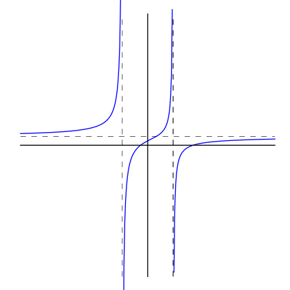 The domain of a function: Graph of a rational function with equation [latex]\frac{(x^2 - 3x -2)}{(x^2 - 4)}[/latex]. The domain of this function is all values of [latex]x[/latex] except [latex]+2[/latex] or [latex]-2[/latex].
Example 2
Consider the rational function [latex-display]f(x)= \dfrac{(x + 3)}{(x^2 + 2)}[/latex-display] The domain of this function is all values of [latex]x[/latex] except those where [latex]x^2 + 2 = 0[/latex]. However, for [latex]x^2 + 2=0[/latex], [latex]x^2[/latex] would need to equal [latex]-2[/latex]. Since this condition cannot be satisfied by a real number, the domain of the function is all real numbers.Asymptotes
A rational function can have at most one horizontal or oblique asymptote, and many possible vertical asymptotes; these can be calculated.Learning Objectives
Determine when the asymptote of a rational function will be horizontal, oblique, or verticalKey Takeaways
Key Points
- An asymptote of a curve is a line, such that the distance between the curve and the line approaches zero as they tend to infinity.
- There are three kinds of asymptotes: horizontal, vertical and oblique.
- A rational function has at most one horizontal asymptote or oblique (slant) asymptote, and possibly many vertical asymptotes.
- Vertical asymptotes occur at singularities of a rational function, or points at which the function is not defined. They only occur at singularities where the associated linear factor in the denominator remains after cancellation.
- The existence of a horizontal or oblique asymptote depends on the degrees of polynomials in the numerator and denominator.
Key Terms
- asymptote: A straight line which a curve approaches arbitrarily closely, as it goes to infinity.
- oblique: Not erect or perpendicular; neither parallel to, nor at right angles from, the base; slanting; inclined.
- rational function: Any function whose value can be expressed as the quotient of two polynomials (where the polynomial in the denominator is not zero).
Types of Asymptotes
In analytic geometry, an asymptote of a curve is a line such that the distance between the curve and the line approaches zero as they tend to infinity. There are three kinds of asymptotes: horizontal, vertical and oblique. Horizontal asymptotes of curves are horizontal lines that the graph of the function approaches as [latex]x[/latex] tends to [latex]+ \infty[/latex] or [latex]- \infty[/latex]. Horizontal asymptotes are parallel to the [latex]x[/latex]-axis. Vertical asymptotes are vertical lines near which the function grows without bound. They are parallel to the [latex]y[/latex]-axis. An asymptote that is neither horizontal or vertical is an oblique (or slant) asymptote. These are diagonal lines so that the difference between the curve and the line approaches [latex]0[/latex] as [latex]x[/latex] tends to [latex]+ \infty[/latex] or [latex]- \infty[/latex]. Each type of asymptote is shown in the graph below.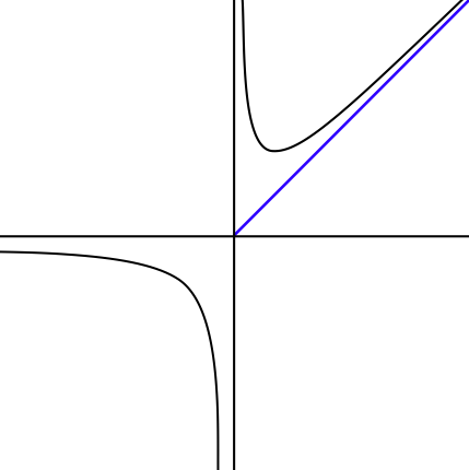 Graph with asymptotes: The graph of a function with a horizontal ([latex]y=0[/latex]), vertical ([latex]x=0[/latex]), and oblique asymptote (blue line).
Example 1
Consider the graph of the equation [latex]f(x) = \frac {1}{x}[/latex], shown below. The coordinates of the points on the curve are of the form [latex](x, \frac {1}{x})[/latex] where [latex]x[/latex] is a number other than 0.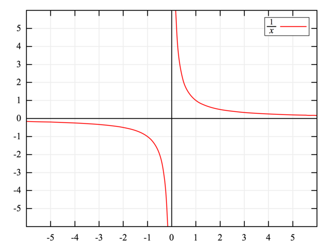 Graph of [latex]f(x) = 1/x[/latex]: Both the [latex]x[/latex]-axis and [latex]y[/latex]-axis are asymptotes.
Asymptotes of Rational Functions
A rational function has at most one horizontal or oblique asymptote, and possibly many vertical asymptotes. Vertical asymptotes occur only when the denominator is zero. In other words, vertical asymptotes occur at singularities, or points at which the rational function is not defined. Vertical asymptotes only occur at singularities when the associated linear factor in the denominator remains after cancellation. For example, consider the function: [latex-display]f(x) = \dfrac{(x-1)(x+2)}{(x-1)(x+1)}[/latex-display] We can identify from the linear factors in the denominator that two singularities exist, at [latex]x=1[/latex] and [latex]x = -1[/latex]. However, the linear factor [latex](x-1)[/latex] cancels with a factor in the numerator. Thus, the only vertical asymptote for this function is at [latex]x=-1[/latex]. The degree of the numerator and degree of the denominator determine whether or not there are any horizontal or oblique asymptotes. Existence of horizontal asymptote depends on the degree of polynomial in the numerator ([latex]n[/latex]) and degree of polynomial in the denominator ([latex]m[/latex]). There are three possible cases:- If [latex]n>m[/latex], then there is no horizontal asymptote (However, if [latex]n = m+1[/latex], then there exists a slant asymptote).
- If [latex]n<m[/latex], then the [latex]x[/latex]-axis is a horizontal asymptote.
- If [latex]n=m[/latex], then a horizontal asymptote exists, and the equation is:
Example 2
Find any vertical asymptotes of [latex]f(x) = \dfrac{(x-1)(x+2)}{(x-1)^2(x+1)}[/latex]. Notice that, based on the linear factors in the denominator, singularities exists at [latex]x=1[/latex] and [latex]x=-1[/latex]. Also notice that one linear factor [latex](x-1)[/latex] cancels with the numerator. However, one linear factor [latex](x-1)[/latex] remains in the denominator because it is squared. Therefore, a vertical asymptote exists at [latex]x=1[/latex]. The linear factor [latex](x + 1)[/latex] also does not cancel out; thus, a vertical asymptote also exists at [latex]x = -1[/latex].Example 3
Find any horizontal or oblique asymptote of [latex]f(x) = \dfrac{2x^2 + x + 1}{x^2 + 16}[/latex]. Because the polynomials in the numerator and denominator have the same degree ([latex]2[/latex]), we can identify that there is one horizontal asymptote and no oblique asymptote. The coefficient of the highest power term is [latex]2[/latex] in the numerator and [latex]1[/latex] in the denominator. Hence, horizontal asymptote is given by: [latex-display]y = \frac{2}{1} = 2[/latex-display]Solving Problems with Rational Functions
The [latex]x[/latex]-intercepts of rational functions are found by setting the polynomial in the numerator equal to [latex]0[/latex] and solving for [latex]x[/latex].Learning Objectives
Use the numerator of a rational function to solve for its zerosKey Takeaways
Key Points
- The [latex]x[/latex]-intercepts (also known as zeros or roots ) of a function are points where the graph intersects the [latex]x[/latex]-axis. Rational functions can have zero, one, or multiple [latex]x[/latex]-intercepts.
- For any function, the [latex]x[/latex]-intercepts are [latex]x[/latex]-values for which the function has a value of zero: [latex]f(x) = 0[/latex].
- For rational functions, the [latex]x[/latex]-intercepts exist when the numerator is equal to [latex]0[/latex]. For [latex]f(x) = \frac{P(x)}{Q(x)}[/latex], if [latex]P(x) = 0[/latex], then [latex]f(x) = 0[/latex].
Key Terms
- denominator: The number or expression written below the line in a fraction (thus [latex]2[/latex] in [latex]\frac {1}{2}[/latex]).
- rational function: Any function whose value can be expressed as the quotient of two polynomials (except division by zero).
- numerator: The number or expression written above the line in a fraction (thus [latex]1[/latex] in [latex]\frac {1}{2}[/latex]).
Finding the [latex]x[/latex]-intercepts of Rational Functions
Recall that a rational function is defined as the ratio of two real polynomials with the condition that the polynomial in the denominator is not a zero polynomial. [latex-display]f(x) = \dfrac{P(x)}{Q(x)}[/latex], where [latex]Q(x) \neq 0[/latex-display] An example of a rational function is: [latex-display]f(x) = \dfrac{x + 1}{2x^2 - x - 1}[/latex-display] Rational functions can be graphed on the coordinate plane. We can use algebraic methods to calculate their [latex]x[/latex]-intercepts (also known as zeros or roots), which are points where the graph intersects the [latex]x[/latex]-axis. Rational functions can have zero, one, or multiple [latex]x[/latex]-intercepts. For any function, the [latex]x[/latex]-intercepts are [latex]x[/latex]-values for which the function has a value of zero: [latex]f(x) = 0[/latex]. In the case of rational functions, the [latex]x[/latex]-intercepts exist when the numerator is equal to [latex]0[/latex]. For [latex]f(x) = \frac{P(x)}{Q(x)}[/latex], if [latex]P(x) = 0[/latex], then [latex]f(x) = 0[/latex]. In order to solve rational functions for their [latex]x[/latex]-intercepts, set the polynomial in the numerator equal to zero, and solve for [latex]x[/latex] by factoring where applicable.Example 1
Find the [latex]x[/latex]-intercepts of this function: [latex-display]f(x) = \dfrac{x^2 - 3x + 2}{x^2 - 2x -3}[/latex-display] Set the numerator of this rational function equal to zero and solve for [latex]x[/latex]: [latex]\begin {align} 0 &=x^2 - 3x + 2 \\&= (x - 1)(x - 2) \end {align}[/latex] Solutions for this polynomial are [latex]x = 1[/latex] or [latex]x= 2[/latex]. This means that this function has [latex]x[/latex]-intercepts at [latex]1[/latex] and [latex]2[/latex].Example 2
Find the [latex]x[/latex]-intercepts of the function: [latex-display]f(x) = \dfrac {1}{x}[/latex-display] Here, the numerator is a constant, and therefore, cannot be set equal to [latex]0[/latex]. Thus, this function does not have any [latex]x[/latex]-intercepts.Example 3
Find the roots of: [latex-display]g(x) = \dfrac{x^3 - 2x}{2x^2 - 10} [/latex-display] Factoring the numerator, we have: [latex]\begin {align} 0&=x^3 - 2x \\&= x(x^2 - 2) \end {align}[/latex] Given the factor [latex]x[/latex], the polynomial equals [latex]0[/latex] when [latex]x=0[/latex]. Let the second factor equal zero, and solve for [latex]x[/latex]: [latex]x^2 - 2 = 0 \\ x^2 = 2 \\ x = \pm \sqrt{2}[/latex] Thus there are three roots, or [latex]x[/latex]-intercepts: [latex]0[/latex], [latex]-\sqrt{2}[/latex] and [latex]\sqrt{2}[/latex]. These can be observed in the graph of the function below.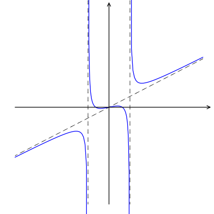 Graph of [latex]g(x) = \frac{x^3 - 2x}{2x^2 - 10}[/latex]: [latex]x[/latex]-intercepts exist at [latex]x = -\sqrt{2}, 0, \sqrt{2}[/latex].
Simplifying, Multiplying, and Dividing Rational Expressions
A rational expression can be treated like a fraction, and can be manipulated via multiplication and division.Learning Objectives
Practice simplifying, multiplying, and dividing rational expressionsKey Takeaways
Key Points
- A rational expression is a quotient of two polynomials, where the polynomial in the denominator is not zero.
- Rational expressions can often be simplified by removing terms that can be factored out of the numerator and denominator. These can be either numbers or functions of [latex]x[/latex].
- Rational expressions can be multiplied together. The numerators of each are multiplied together, as well as their denominators. Sometimes, it is possible to simplify the resulting fraction.
- Rational expressions can be divided by one another. This follows the rules for dividing fractions, where the dividend is multiplied by the reciprocal of the divisor.
Key Terms
- expression: An arrangement of symbols denoting values, operations performed on them, and grouping symbols, e.g. [latex]\displaystyle \frac{(2x+4)}{2}[/latex]
- rational expression: An expression that can be expressed as the quotient of two polynomials, where the polynomial in the denominator is not zero.
- polynomial: An expression consisting of a sum of a finite number of terms, each term being the product of a constant coefficient and one or more variables raised to a non-negative integer power, such as [latex]a_n x^n + a_{n-1}x^{n-1} +... + a_0 x^0[/latex]. Importantly, because all exponents are positive, it is impossible to divide by [latex]x[/latex].
Simplifying a Rational Expression
Rational expressions can be simplified by factoring the numerator and denominator where possible, and canceling terms. As a first example, consider the rational expression [latex]\frac { 3x^3 }{ x }[/latex]. This can be simplified by canceling out one factor of [latex]x[/latex] in the numerator and denominator, which gives the expression [latex]3x^2[/latex]. Note that the domain of the equation [latex]f(x) = \frac{3x^3}{x}[/latex] does not include [latex]x=0[/latex], as this would cause division by [latex]0[/latex]. The latter form is a simplified version of the former graphically. Consider a more complicated example: [latex-display]\displaystyle \frac { x^2+5x+6 }{ 2x^2+5x+2 }[/latex-display] This expression must first be factored to provide the expression [latex-display]\displaystyle \frac {(x+2)(x+3)}{(2x+1)(x+2)}[/latex-display] which, after canceling the common factor of [latex](x+2)[/latex] from both the numerator and denominator, gives the simplified expression [latex-display]\displaystyle \frac {x+3}{2x+1}[/latex-display]Multiplying Rational Expressions
Rational expressions can be multiplied and divided in a similar manner to fractions. Recall that when two fractions are multiplied together, their numerators are multiplied to yield the numerator of their product, and their denominators are multiplied to yield the denominator of their product. For a simple example, consider the following, where a rational expression is multiplied by a fraction of whole numbers: [latex-display]\displaystyle \frac {x^2+3}{2x-3} \times \frac{2}{3}[/latex-display] Following the rule for multiplying fractions, simply multiply their respective numerators and denominators: [latex-display]\displaystyle \frac {2(x^2+3)}{3(2x-3)}[/latex-display] This can be multiplied through to yield [latex]\displaystyle \frac {2x^2+6}{6x-9}[/latex] Notice that we multiplied the numerators together and the denominators together, but we did not multiply the numerator by the denominator or vice-versa. We follow the same rules to multiply two rational expressions together. The operations are slightly more complicated, as there may be a need to simplify the resulting expression.Example 1
Consider the following: [latex-display]\displaystyle \frac {x+1}{x-1} \times \frac {x+2}{x+3}[/latex-display] Multiplying these two expressions, we have the product: [latex-display]\displaystyle\frac {(x+1)(x+2)}{(x-1)(x+3)}[/latex-display] Multiplying out the numerator and denominator, this can be written as: [latex-display]\displaystyle \frac {x^2+3x+2}{x^2+2x-3}[/latex-display] Notice that this expression cannot be simplified further.Dividing Rational Expressions
Dividing rational expressions follows the same rules as dividing fractions. Recall the rule for dividing fractions: the dividend is multiplied by the reciprocal of the divisor. The same applies to dividing rational expressions; the first expression is multiplied by the reciprocal of the second.Example 2
Consider the following: [latex-display]\displaystyle \frac {x+1}{x-1} \div \frac {x+2}{x+3}[/latex-display] Rather than divide the expressions, we multiply [latex]\displaystyle \frac {x+1}{x-1}[/latex] by the reciprocal of [latex]\displaystyle \frac {x+2}{x+3}[/latex]: [latex-display]\displaystyle \frac{x+1}{x-1} \times \frac {x+3}{x+2}[/latex-display] Then, multiplication is carried out in the same way as described above: [latex-display]\displaystyle \frac{(x+1)(x+3)}{(x-1)(x+2)} = \frac{x^2 + 3x +3}{x^2 + x - 2}[/latex-display] The expression cannot be simplified further.Partial Fractions
Partial fraction decomposition is a procedure used to reduce the degree of either the numerator or the denominator of a rational function.Learning Objectives
Practice breaking a rational function into partial fractionsKey Takeaways
Key Points
- Partial fraction decomposition is a procedure used to reduce the degree of either the numerator or the denominator of a rational function, and involves splitting one ratio up into multiple simpler ratios. In mathematical terms, partial fraction decomposition turns a function of the form [latex]\frac{f(x)}{g(x)}[/latex], where [latex]f[/latex] and [latex]g[/latex] are both polynomials, into a function of the form [latex]\sum_{j}\frac{f_{j}(x)}{g_{j}(x)}[/latex], where [latex]g_{j}(x)[/latex] are polynomials that are factors of [latex]g(x)[/latex].
- The main motivation to decompose a rational function into a sum of simpler fractions is to make it simpler to perform linear operations on the sum.
- There are special cases that cannot be solved by the methodology described here. These include rational functions with repeated roots, and those where the degree of the polynomial in the numerator is greater than or equal to that in the denominator.
Key Terms
- degree: the sum of the exponents of a term; the order of a polynomial.
- polynomial: an expression consisting of a sum of a finite number of terms, each term being the product of a constant coefficient and one or more variables raised to a non-negative integer power, such as [latex]a_n x^n + a_{n-1}x^{n-1} +... + a_0 x^0[/latex]. Importantly, because all exponents are positive, it is impossible to divide by [latex]x[/latex].
Partial Fraction Decomposition
In algebra, partial fraction decomposition (sometimes called partial fraction expansion) is a procedure used to reduce the degree of either the numerator or the denominator of a rational function. It involves splitting one ratio up into multiple simpler ratios. Here's an example of one ratio being split into a sum of three simpler ratios: [latex]\displaystyle \frac{8x^2 + 3x - 21}{x^3 -7x -6} = \frac{1}{x+2} + \frac{3}{x-3} + \frac{4}{x+1}[/latex] In mathematical terms, partial fraction expansion is used to change a rational function in the form [latex]\frac{f(x)}{g(x)}[/latex], where [latex]f[/latex] and [latex]g[/latex] are polynomials, into a function of the form [latex]\sum_{j}\frac{f_{j}(x)}{g_{j}(x)}[/latex]. The denominators of the terms of this summation, [latex]g_{j}(x)[/latex], are polynomials that are factors of [latex]g(x)[/latex], and in general are of lower degree. The main motivation to decompose a rational function into a sum of simpler fractions is to make it easier to perform linear operations on the sum. Reducing complex mathematical problems via partial fraction decomposition allows us to focus on computing each single element of the decomposition rather than the more complex rational function.Steps to Decomposing a Rational Function
Say we have a rational function [latex]R(x) = \frac{f(x)}{g(x)}[/latex], where the degree of the numerator is less than the degree of the denominator. Assume [latex]R(x)[/latex] has a denominator that factors into other expressions, as [latex]g(x)=P(x)\cdot Q(x)[/latex], and that there are no repeated roots. The first step to decomposing the function [latex]R(x)[/latex] is to factor its denominator: [latex-display]\displaystyle R(x) = \frac{f(x)}{(x - a_1)(x - a_2)\cdots (x - a_p)}[/latex-display] where [latex]a_1,..., a_p[/latex] are the roots of [latex]g(x)[/latex]. We can then write [latex]R(x)[/latex] as the sum of partial fractions: [latex]R(x) = \frac{c_1}{(x - a_1)}+ \frac{c_2}{(x - a_2)}+ \cdots + \frac{c_p}{(x - a_p)}[/latex] where [latex]c_1,..., c_p[/latex] are constants. To complete the process, we must determine the values of these [latex]c_i[/latex] coefficients. To find a coefficient, multiply the denominator associated with it by the rational function [latex]R(x)[/latex]: [latex-display]c_i = (x - a_i)R(x)[/latex-display] This will yield an expression with an [latex]x[/latex]-value. Substitute the associated root [latex]a_i[/latex] in for [latex]x[/latex], and solve for the constant. The following problems provide an examples of this technique.Example 1
Apply decomposition to the rational function [latex]f(x)=\frac{1}{x^{2}+2x-3}[/latex] Factoring the denominator, we have: [latex-display]x^{2}+2x-3=(x+3)(x-1)[/latex-display] So we have the partial fraction decomposition: [latex-display]f(x)=\frac{1}{x^{2}+2x-3}=\frac{c_1}{x+3}+\frac{c_2}{x-1}[/latex-display] Now let's solve for the constant [latex]c_1[/latex]: [latex-display]c_1 = \frac{1}{x^{2}+2x-3} (x+3) = \frac{x+3}{(x+3)(x-1)} = \frac{1}{x-1}[/latex-display] Substituting [latex]x=-3[/latex] into this equation gives [latex]c_1 = -\frac{1}{4}[/latex]. Use the same process to solve for [latex]c_2[/latex]: [latex-display]c_2 = \frac{1}{x^{2}+2x-3} (x-1) = \frac{x-1}{(x+3)(x-1)} = \frac{1}{x+3}[/latex-display] Substituting [latex]x=1[/latex] gives [latex]c_2 = \frac{1}{4}[/latex]. Substituting these coefficients into the decomposed function, we have: [latex]f(x)=\frac{1}{x^{2}+2x-3}=\frac{1}{4}(\frac{-1}{x+3}+\frac{1}{x-1})[/latex]. We have rewritten the initial rational function in terms of partial fractions. This is the most simplified form possible, so we are finished.Example 2
Apply decomposition to the rational function [latex]g(x) = \frac{8x^2 + 3x - 21}{x^3 - 7x - 6}[/latex] Factoring the denominator, we have: [latex-display]x^3 - 7x - 6=(x+2)(x-3)(x+1)[/latex-display] So we have the partial fraction decomposition: [latex-display]g(x)=\frac{8x^2 + 3x - 21}{x^3 - 7x - 6}=\frac{c_1}{(x+2)} + \frac{c_2}{(x-3)}+ \frac{c_3}{(x+1)}[/latex-display] We will now solve for each constant [latex]c_i[/latex]: [latex-display]c_1 = \frac{8x^2 + 3x - 21}{x^3 - 7x - 6} (x+2) = \frac{8x^2 + 3x - 21}{(x-3)(x+1)} [/latex-display] Substituting [latex]x=-2[/latex], we have: [latex]\begin {align} c_1 &= \frac{8(-2)^2 + 3(-2) - 21}{(-2-3)(-2+1)} \\&= \frac {32-27}{(-5)(-1)} \\&=1 \end {align}[/latex] [latex-display]c_2 = \frac{8x^2 + 3x - 21}{x^3 - 7x - 6} (x-3) = \frac{8x^2 + 3x - 21}{(x+2)(x+1)} [/latex-display] Substituting [latex]x=3[/latex], we have: [latex]\begin {align} c_2 &= \frac{8(3)^2 + 3(3) - 21}{(3+2)(3+1)} \\&= \frac {72-12}{15} \\&= 4 \end {align}[/latex] [latex-display]c_3 = \frac{8x^2 + 3x - 21}{x^3 - 7x - 6} (x+1) = \frac{8x^2 + 3x - 21}{(x+2)(x-3)} [/latex-display] Substituting [latex]x=-1[/latex], we have: [latex]\begin {align} c_3&=\frac{8(-1)^2 + 3(-1) - 21}{(-1+2)(-1-3)} \\ &= \frac {8-24}{-4} \\ &= 4 \end {align}[/latex] We have solved for each constant and have our partial fraction expansion: [latex-display]g(x)=\frac{8x^2 + 3x - 21}{x^3 - 7x - 6}=\frac{1}{(x+2)} + \frac{4}{(x-3)}+ \frac{4}{(x+1)}[/latex-display]Additional Considerations
There are some important cases to note, for which partial fraction decomposition becomes more complicated. Decomposition in each of the below cases involves steps in addition to those described above.- If there are repeated roots in the denominator of a rational function (for example, consider [latex]G(x) = \frac{x+2}{(x-1)^2(x+3)}[/latex], for which [latex]x=1[/latex] is a repeated root), additional steps must be taken to decompose the function.
- For a rational function [latex]R(x) = \frac{f(x)}{g(x)}[/latex], if the degree of [latex]f(x)[/latex] is greater than or equal to the degree of [latex]g(x)[/latex], the function cannot be decomposed in a straightforward way. It is necessary to perform the Euclidean division of [latex]f[/latex] by [latex]g[/latex] using polynomial long division, giving [latex]f(x) = E(X)g(x) + h(x)[/latex]. Dividing through by [latex]g(x)[/latex] gives [latex]\frac{f(x)}{g(x)}=E(x)+\frac{h(x)}{g(x)}[/latex], which you can then perform the decomposition on [latex]\frac{h(x)}{g(x)}[/latex].
Licenses & Attributions
CC licensed content, Shared previously
- Curation and Revision. Authored by: Boundless.com. License: Public Domain: No Known Copyright.
CC licensed content, Specific attribution
- Pradnya Bhawalkar and Kim Johnston, Finding the Domain of Simple Rational Functions. September 17, 2013. Provided by: OpenStax CNX Located at: https://cnx.org/contents/0f6f4830-7417-46b5-813b-4d4bd71f5f35@7. License: CC BY: Attribution.
- Rational function. Provided by: Wikipedia Located at: https://en.wikipedia.org/wiki/Rational_function. License: CC BY-SA: Attribution-ShareAlike.
- domain. Provided by: Wiktionary License: CC BY-SA: Attribution-ShareAlike.
- denominator. Provided by: Wiktionary License: CC BY-SA: Attribution-ShareAlike.
- Asymptote. Provided by: Wiktionary License: CC BY-SA: Attribution-ShareAlike.
- Sunil Kumar Singh, Rational function. Provided by: OpenStax CNX Located at: https://cnx.org/contents/9f3c7c3a-e03a-45e3-895e-3ab70bb65e21@10.. License: CC BY: Attribution.
- rational function. Provided by: Wiktionary License: CC BY-SA: Attribution-ShareAlike.
- RationalDegree2byXedi.svg. Provided by: Wikipedia License: CC BY-SA: Attribution-ShareAlike.
- asymptote. Provided by: Wiktionary License: CC BY-SA: Attribution-ShareAlike.
- rational function. Provided by: Wiktionary License: CC BY-SA: Attribution-ShareAlike.
- Asymptote. Provided by: Wikipedia License: CC BY-SA: Attribution-ShareAlike.
- oblique. Provided by: Wiktionary License: CC BY-SA: Attribution-ShareAlike.
- Sunil Kumar Singh, Rational function.. Provided by: OpenStax CNX Located at: https://cnx.org/contents/9f3c7c3a-e03a-45e3-895e-3ab70bb65e21@10. License: CC BY: Attribution.
- RationalDegree2byXedi.svg. Provided by: Wikipedia License: CC BY-SA: Attribution-ShareAlike.
- 1-over-x-plus-x_abs.svg. Provided by: Wikipedia License: CC BY-SA: Attribution-ShareAlike.
- Hyperbola_one_over_x.svg. Provided by: Wikipedia License: CC BY-SA: Attribution-ShareAlike.
- rational function. Provided by: Wiktionary License: CC BY-SA: Attribution-ShareAlike.
- Sunil Kumar Singh, Rational Function. September 17, 2013. Provided by: OpenStax CNX Located at: https://cnx.org/contents/9f3c7c3a-e03a-45e3-895e-3ab70bb65e21@10. License: CC BY: Attribution.
- numerator. Provided by: Wiktionary Located at: https://en.wiktionary.org/wiki/numerator. License: CC BY-SA: Attribution-ShareAlike.
- denominator. Provided by: Wiktionary License: CC BY-SA: Attribution-ShareAlike.
- RationalDegree2byXedi.svg. Provided by: Wikipedia License: CC BY-SA: Attribution-ShareAlike.
- 1-over-x-plus-x_abs.svg. Provided by: Wikipedia License: CC BY-SA: Attribution-ShareAlike.
- Hyperbola_one_over_x.svg. Provided by: Wikipedia License: CC BY-SA: Attribution-ShareAlike.
- RationalDegree3.svg. Provided by: Wikipedia License: Public Domain: No Known Copyright.
- Rational function. Provided by: Wikipedia License: CC BY-SA: Attribution-ShareAlike.
- polynomial. Provided by: Wiktionary License: CC BY-SA: Attribution-ShareAlike.
- expression. Provided by: Wiktionary License: CC BY-SA: Attribution-ShareAlike.
- Boundless. Provided by: Boundless Learning License: CC BY-SA: Attribution-ShareAlike.
- RationalDegree2byXedi.svg. Provided by: Wikipedia Located at: https://en.wikipedia.org/wiki/Rational_function. License: CC BY-SA: Attribution-ShareAlike.
- 1-over-x-plus-x_abs.svg. Provided by: Wikipedia License: CC BY-SA: Attribution-ShareAlike.
- Hyperbola_one_over_x.svg. Provided by: Wikipedia License: CC BY-SA: Attribution-ShareAlike.
- RationalDegree3.svg. Provided by: Wikipedia License: Public Domain: No Known Copyright.
- Partial fraction. Provided by: Wikipedia License: CC BY-SA: Attribution-ShareAlike.
- polynomial. Provided by: Wiktionary License: CC BY-SA: Attribution-ShareAlike.
- degree. Provided by: Wiktionary License: CC BY-SA: Attribution-ShareAlike.
- Thanos Antoulas, JP Slavinsky, Partial Fraction Expansion. Provided by: OpenStax Located at: https://cnx.org/contents/b2e3f8ad-9e60-4421-a343-97e64192ffce@15. License: Public Domain: No Known Copyright.
- RationalDegree2byXedi.svg. Provided by: Wikipedia License: CC BY-SA: Attribution-ShareAlike.
- 1-over-x-plus-x_abs.svg. Provided by: Wikipedia License: CC BY-SA: Attribution-ShareAlike.
- Hyperbola_one_over_x.svg. Provided by: Wikipedia License: CC BY-SA: Attribution-ShareAlike.
- RationalDegree3.svg. Provided by: Wikipedia License: Public Domain: No Known Copyright.
