Introduction to Matrices
What is a Matrix?
A matrix is a rectangular arrays of numbers, symbols, or expressions, arranged in rows and columns.
Learning Objectives
Describe the parts of a matrix and what they represent
Key Takeaways
Key Points
- A matrix (whose plural is matrices) is a rectangular array of numbers, symbols, or expressions, arranged in rows and columns.
- A matrix with [latex]m[/latex] rows and [latex]n[/latex] columns is called an [latex]m\times n[/latex] matrix or [latex]m[/latex]-by-[latex]n[/latex] matrix, where [latex]m[/latex] and [latex]n[/latex] are called the matrix dimensions.
- Matrices can be used to compactly write and work with multiple linear equations, that is, a system of linear equations. Matrices and matrix multiplication reveal their essential features when related to linear transformations, also known as linear maps.
Key Terms
- element: An individual item in a matrix
- row vector: A matrix with a single row
- column vector: A matrix with a single column
- square matrix: A matrix which has the same number of rows and columns
- matrix: A rectangular array of numbers, symbols, or expressions, arranged in rows and columns
History of the Matrix
The matrix has a long history of application in solving linear equations. They were known as arrays until the [latex]1800[/latex]'s. The term "matrix" (Latin for "womb", derived from mater—mother) was coined by James Joseph Sylvester in [latex]1850[/latex], who understood a matrix as an object giving rise to a number of determinants today called minors, that is to say, determinants of smaller matrices that are derived from the original one by removing columns and rows. An English mathematician named Cullis was the first to use modern bracket notation for matrices in [latex]1913[/latex] and he simultaneously demonstrated the first significant use of the notation [latex]A=a_{i,j}[/latex] to represent a matrix where [latex]a_{i,j}[/latex] refers to the element found in the ith row and the jth column. Matrices can be used to compactly write and work with multiple linear equations, referred to as a system of linear equations, simultaneously. Matrices and matrix multiplication reveal their essential features when related to linear transformations, also known as linear maps.
What is a Matrix
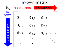
In mathematics, a matrix (plural matrices) is a rectangular array of numbers, symbols, or expressions, arranged in rows and columns. Matrices are commonly written in box brackets. The horizontal and vertical lines of entries in a matrix are called rows and columns, respectively. The size of a matrix is defined by the number of rows and columns that it contains. A matrix with m rows and n columns is called an m × n matrix or [latex]m[/latex]-by-[latex]n[/latex] matrix, while m and n are called its dimensions.The dimensions of the following matrix are [latex]2 \times 3[/latex] up(read "two by three"), because there are two rows and three columns.
[latex-display]A={\displaystyle {\begin{bmatrix}1&9&-13\\20&5&-6\end{bmatrix}}}[/latex-display]
 Matrix Dimensions:
 Each element of a matrix is often denoted by a variable with two subscripts. For instance, [latex]a_{2,1}[/latex] represents the element at the second row and first column of a matrix A.
Addition and Subtraction; Scalar Multiplication
Matrix addition, subtraction, and scalar multiplication are types of operations that can be applied to modify matrices.
Learning Objectives
Practice adding and subtracting matrices, as well as multiplying matrices by scalar numbers
Key Takeaways
Key Points
- When performing addition, add each element in the first matrix to the corresponding element in the second matrix.
- When performing subtraction, subtract each element in the second matrix from the corresponding element in the first matrix.
- Addition and subtraction require that the matrices be the same dimensions. The resultant matrix is also of the same dimension.
- Scalar multiplication of a real Euclidean vector by a positive real number multiplies the magnitude of the vector without changing its direction.
Key Terms
- scalar: A quantity that has magnitude but not direction.
There are a number of operations that can be applied to modify matrices, such as matrix addition, subtraction, and scalar multiplication. These form the basic techniques to work with matrices.
These techniques can be used in calculating sums, differences and products of information such as sodas that come in three different flavors: apple, orange, and strawberry and two different packaging: bottle and can. Two tables summarizing the total sales between last month and this month are written to illustrate the amounts. Matrix addition, subtraction and scalar multiplication can be used to find such things as: the sales of last month and the sales of this month, the average sales for each flavor and packaging of soda in the [latex]2[/latex]-month period.
Adding and Subtracting Matrices
We use matrices to list data or to represent systems. Because the entries are numbers, we can perform operations on matrices. We add or subtract matrices by adding or subtracting corresponding entries.
In order to do this, the entries must correspond. Therefore, addition and subtraction of matrices is only possible when the matrices have the same dimensions. Matrix addition is commutative and is also associative, so the following is true:
[latex]\displaystyle
A+B=B+A
[/latex]
[latex]\displaystyle
(A+B)+C=A+(B+C)[/latex]
Adding matrices is very simple. Just add each element in the first matrix to the corresponding element in the second matrix.
[latex]\displaystyle
\begin {pmatrix} 1 & 2 & 3 \\ 4 & 5 & 6 \end{pmatrix}+\begin{pmatrix} 10 & 20 & 30 \\ 40 & 50 & 60 \end{pmatrix}=\begin {pmatrix} 11 & 22 & 33 \\ 44 & 55 & 66 \end {pmatrix}[/latex]
Note that element in the first matrix, [latex]1[/latex], adds to element [latex]x_{11}[/latex] in the second matrix, [latex]10[/latex], to produce element [latex]x_{11}[/latex] in the resultant matrix, [latex]11[/latex]. Also note that both matrices being added are [latex]2\times 3[/latex], and the resulting matrix is also [latex]2\times 3[/latex]. You cannot add two matrices that have different dimensions.
As you might guess, subtracting works much the same way except that you subtract instead of adding.
[latex]\displaystyle
\begin{pmatrix} 10 & -20 & 30 \\ 40 & 50 & 60 \end{pmatrix}-\begin{pmatrix} 1 & -2 & 3 \\ 4 & -5 & 6 \end{pmatrix}=\begin{pmatrix} 9 & -18 & 27 \\ 36 & 55 & 54 \end{pmatrix}[/latex]
Once again, note that the resulting matrix has the same dimensions as the originals, and that you cannot subtract two matrices that have different dimensions. Be careful when subtracting with signed numbers.
Scalar Multiplication
In an intuitive geometrical context, scalar multiplication of a real Euclidean vector by a positive real number multiplies the magnitude of the vector without changing its direction. What does it mean to multiply a number by [latex]3[/latex]? It means you add the number to itself [latex]3[/latex] times. Multiplying a matrix by [latex]3[/latex] means the same thing; you add the matrix to itself [latex]3[/latex] times, or simply multiply each element by that constant.
[latex]\displaystyle
3\cdot \begin{pmatrix} 1 & 2 & 3 \\ 4 & 5 & 6 \end{pmatrix}=\begin{pmatrix} 3 & 6 & 9 \\ 12 & 15 & 18 \end{pmatrix}[/latex]
The resulting matrix has the same dimensions as the original. Scalar multiplication has the following properties:
- Left and right distributivity: [latex](c+d)\textbf{M} = \textbf{M}(c+d) = \textbf{M}c+\textbf{M}d[/latex]
- Associativity: [latex](cd)\textbf{M} = c(d\textbf{M})[/latex]
- Identity: [latex]1\textbf{M} = \textbf{M}[/latex]
- Null: [latex]0\textbf{M} = \textbf{0}[/latex]
- Additive inverse: [latex](-1)\textbf{M} = -\textbf{M}[/latex]
Matrix Multiplication
When multiplying matrices, the elements of the rows in the first matrix are multiplied with corresponding columns in the second matrix.
Learning Objectives
Practice multiplying matrices and identify matrices that can be multiplied together
Key Takeaways
Key Points
- If [latex]A[/latex] is an [latex]n\times m [/latex] matrix and [latex]B[/latex] is an [latex]m \times p[/latex] matrix, the result [latex]AB[/latex] of their multiplication is an [latex]n \times p[/latex] matrix defined only if the number of columns [latex]m[/latex] in [latex]A[/latex] is equal to the number of rows [latex]m[/latex] in [latex]B[/latex].
- The product of a square matrix multiplied by a column matrix arises naturally in linear algebra for solving linear equations and representing linear transformations.
Key Terms
- matrix: A rectangular arrangement of numbers or terms having various uses such as transforming coordinates in geometry, solving systems of linear equations in linear algebra and representing graphs in graph theory.
If [latex]A[/latex] is an [latex]n\times m [/latex] matrix and [latex]B[/latex] is an [latex]m \times p[/latex] matrix, the result [latex]AB[/latex] of their multiplication is an [latex]n \times p[/latex] matrix defined only if the number of columns [latex]m[/latex] in [latex]A[/latex] is equal to the number of rows [latex]m[/latex] in [latex]B[/latex]. Check to make sure that this is true before multiplying the matrices, since there is "no solution" otherwise.
General Definition and Process: Matrix Multiplication
Scalar multiplication is simply multiplying a value through all the elements of a matrix, whereas matrix multiplication is multiplying every element of each row of the first matrix times every element of each column in the second matrix. Scalar multiplication is much more simple than matrix multiplication; however, a pattern does exist.
When multiplying matrices, the elements of the rows in the first matrix are multiplied with corresponding columns in the second matrix. Each entry of the resultant matrix is computed one at a time.
For two matrices the final position of the product is shown below:
[latex]\displaystyle
\begin{bmatrix} { a }_{ 11 } & { a }_{ 12 } \\ \cdot & \cdot \\ { a }_{ 31 } & { a }_{ 32 } \\ \cdot & \cdot \end{bmatrix}\begin{bmatrix} \cdot & { b }_{ 12 } & { b }_{ 13 } \\ \cdot & { b }_{ 22 } & { b }_{ 23 } \end{bmatrix}=\begin{bmatrix} \cdot & x_{ 12 } & \cdot \\ \cdot & \cdot & \cdot \\ \cdot & \cdot & { x }_{ 33 } \\ \cdot & \cdot & \cdot \end{bmatrix}[/latex]
 Matrix Multiplication:
 This figure illustrates diagrammatically the product of two matrices A and B, showing how each intersection in the product matrix corresponds to a row of A and a column of B.
Matrix Multiplication: Process
Example 1: Find the product [latex]AB[/latex]
[latex]\displaystyle
A=\begin{pmatrix} { 1 } & { 2 } \\ { 3 } & { 4 } \end{pmatrix}\quad B=\begin{pmatrix} { 5 } & { 6 } \\ { 7 } & { 8 } \end{pmatrix}
[/latex]
First ask: Do the number of columns in [latex]A[/latex] equal the number of rows in [latex]B[/latex]? The number of columns in [latex]A[/latex] is [latex]2[/latex], and the number of rows in [latex]B[/latex] is also [latex]2[/latex], therefore a product exists.
Start with producing the product for the first row, first column element. Take the first row of Matrix [latex]A[/latex] and multiply by the first column of Matrix [latex]B[/latex]: The first element of [latex]A[/latex] times the first column element of [latex]B[/latex], plus the second element of [latex]A[/latex] times the second column element of [latex]B[/latex].
[latex]\displaystyle
AB=\begin{pmatrix} { (1 \cdot 5) }+{ (2 \cdot 7) } & ({ })+{ ( )} \\ { ( ) }+{ ( ) } & { ( ) }+{ ( ) } \end{pmatrix}[/latex]
Continue the pattern with the first row of [latex]A[/latex] by the second column of [latex]B[/latex], and then repeat with the second row of [latex]A[/latex].
AB has entries defined by the equation:
[latex]\displaystyle
AB=\begin{pmatrix} { (1 \cdot 5) }+{ (2 \cdot 7) } & ({ 1 \cdot 6})+{ (2 \cdot 8)} \\ { (3 \cdot 5) }+{ (4 \cdot 7) } & { (3 \cdot 6) }+{ (4 \cdot 8) } \end{pmatrix}[/latex]
[latex]\displaystyle
AB=\begin{pmatrix} {(5+14)} & {(6+16)} \\ {(15+28)} & {(18+32)} \end{pmatrix}[/latex]
[latex]\displaystyle
AB= \begin{pmatrix} {(19)} & {(22)} \\ {(43)} & {(50)} \end{pmatrix}[/latex]
The Identity Matrix
The identity matrix [latex][I][/latex] is defined so that [latex][A][I]=[I][A]=[A][/latex], i.e. it is the matrix version of multiplying a number by one.
Learning Objectives
Discuss the properties of the identity matrix
Key Takeaways
Key Points
- For any square matrix, its identity matrix is a diagonal stretch of [latex]1[/latex]s going from the upper-left-hand corner to the lower-right, with all other elements being [latex]0[/latex].
- Non-square matrices do not have an identity. That is, for a non-square matrix [latex][A][/latex], there is no matrix such that [latex][A][I]=[I][A]=[A][/latex].
- Proving that the identity matrix functions as desired requires the use of matrix multiplication.
Key Terms
- matrix: A rectangular arrangement of numbers or terms having various uses such as transforming coordinates in geometry, solving systems of linear equations in linear algebra and representing graphs in graph theory.
- identity matrix: A diagonal matrix all of the diagonal elements of which are equal to [latex]1[/latex], the rest being equal to [latex]0[/latex].
The number [latex]1[/latex] has a special property: when multiplying any number by [latex]1[/latex], the result is the same number, i.e. [latex]5 \cdot 1 = 5[/latex]. This idea can be expressed with the following property as an algebraic generalization: [latex]1x=x[/latex]. The matrix that has this property is referred to as the identity matrix.
Definition of the Identity Matrix
The identity matrix, designated as [latex][I][/latex], is defined by the property:
[latex]\displaystyle
[A][I]=[I][A]=[A][/latex].
Note that the definition of [I][I] stipulates that the multiplication must commute, that is, it must yield the same answer no matter in which order multiplication is done.
This stipulation is important because, for most matrices, multiplication does not commute.
What matrix has this property? A first guess might be a matrix full of [latex]1[/latex]s, but that does not work:
[latex]\displaystyle
\begin{pmatrix} 1 & 2 \\ 3 & 4 \end{pmatrix} \begin{pmatrix} 1 & 1 \\ 1 & 1 \end{pmatrix} = \begin{pmatrix} 3 & 3 \\ 7 & 7 \end{pmatrix}[/latex]
So [latex]\begin{pmatrix} 1 & 1 \\ 1 & 1 \end{pmatrix}[/latex] is not an identity matrix.
The matrix that does work is a diagonal stretch of [latex]1[/latex]s, with all other elements being [latex]0[/latex].
[latex]\displaystyle
\begin{pmatrix} 1 & 3 \\ 2 & 4 \end{pmatrix} \begin{pmatrix} 1 & 0 \\ 0 & 1 \end{pmatrix} = \begin{pmatrix} 1 & 3 \\ 2 & 4 \end{pmatrix}[/latex]
So [latex]\begin{pmatrix} 1 & 0 \\ 0 & 1 \end{pmatrix}[/latex] is the identity matrix for [latex]2 \times 2[/latex] matrices.
For a [latex]3 \times 3[/latex] matrix, the identity matrix is a [latex]3 \times 3[/latex] matrix with diagonal [latex]1[/latex]s and the rest equal to [latex]0[/latex]:
[latex]\displaystyle
\begin{pmatrix} 2 & \pi & -3 \\ 5 & -2 & \frac 12 \\ 9 & 8 & 8.3 \end{pmatrix} \begin{pmatrix} 1 & 0 & 0 \\ 0 & 1 & 0 \\ 0 & 0 & 1 \end{pmatrix} = \begin{pmatrix} 2 & \pi & -3 \\ 5 & -2 & \frac 12 \\ 9 & 8 & 8.3 \end{pmatrix}[/latex]
So [latex]\begin{pmatrix} 1 & 0 & 0 \\ 0 & 1 & 0 \\ 0 & 0 & 1 \end{pmatrix}[/latex] is the identity matrix for [latex]3 \times 3[/latex] matrices.
It is important to confirm those multiplications, and also confirm that they work in reverse order (as the definition requires).
There is no identity for a non-square matrix because of the requirement of matrices being commutative. For a non-square matrix [latex][A][/latex] one might be able to find a matrix [latex][I][/latex] such that [latex][A][I]=[A][/latex], however, if the order is reversed then an illegal multiplication will be left. The reason for this is because, for two matrices to be multiplied together, the first matrix must have the same number of columns as the second has rows.Licenses & Attributions
CC licensed content, Shared previously
CC licensed content, Specific attribution
