Introduction to Linear Functions
What is a Linear Function?
Linear functions are algebraic equations whose graphs are straight lines with unique values for their slope and y-intercepts.Learning Objectives
Describe the parts and characteristics of a linear functionKey Takeaways
Key Points
- A linear function is an algebraic equation in which each term is either a constant or the product of a constant and (the first power of) a single variable.
- A function is a relation with the property that each input is related to exactly one output.
- A relation is a set of ordered pairs.
- The graph of a linear function is a straight line, but a vertical line is not the graph of a function.
- All linear functions are written as equations and are characterized by their slope and [latex]y[/latex]-intercept.
Key Terms
- relation: A collection of ordered pairs.
- variable: A symbol that represents a quantity in a mathematical expression, as used in many sciences.
- linear function: An algebraic equation in which each term is either a constant or the product of a constant and (the first power of) a single variable.
- function: A relation between a set of inputs and a set of permissible outputs with the property that each input is related to exactly one output.
What is a Linear Function?
A linear function is an algebraic equation in which each term is either a constant or the product of a constant and (the first power of) a single variable. For example, a common equation, [latex]y=mx+b[/latex], (namely the slope-intercept form, which we will learn more about later) is a linear function because it meets both criteria with [latex]x[/latex] and [latex]y[/latex] as variables and [latex]m[/latex] and [latex]b[/latex] as constants. It is linear: the exponent of the [latex]x[/latex] term is a one (first power), and it follows the definition of a function: for each input ([latex]x[/latex]) there is exactly one output ([latex]y[/latex]). Also, its graph is a straight line.Graphs of Linear Functions
The origin of the name "linear" comes from the fact that the set of solutions of such an equation forms a straight line in the plane. In the linear function graphs below, the constant, [latex]m[/latex], determines the slope or gradient of that line, and the constant term, [latex]b[/latex], determines the point at which the line crosses the [latex]y[/latex]-axis, otherwise known as the [latex]y[/latex]-intercept.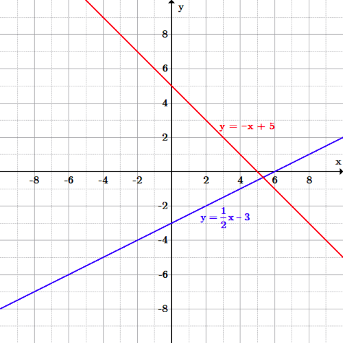 Graphs of linear functions: The blue line, [latex]y=\frac{1}{2}x-3[/latex] and the red line, [latex]y=-x+5[/latex] are both linear functions. The blue line has a positive slope of [latex]\frac{1}{2}[/latex] and a [latex]y[/latex]-intercept of [latex]-3[/latex]; the red line has a negative slope of [latex]-1[/latex] and a [latex]y[/latex]-intercept of [latex]5[/latex].
Vertical and Horizontal Lines
Vertical lines have an undefined slope, and cannot be represented in the form [latex]y=mx+b[/latex], but instead as an equation of the form [latex]x=c[/latex] for a constant [latex]c[/latex], because the vertical line intersects a value on the [latex]x[/latex]-axis, [latex]c[/latex]. For example, the graph of the equation [latex]x=4[/latex] includes the same input value of [latex]4[/latex] for all points on the line, but would have different output values, such as [latex](4,-2),(4,0),(4,1),(4,5),[/latex] etcetera. Vertical lines are NOT functions, however, since each input is related to more than one output. Horizontal lines have a slope of zero and is represented by the form, [latex]y=b[/latex], where [latex]b[/latex] is the [latex]y[/latex]-intercept. A graph of the equation [latex]y=6[/latex] includes the same output value of 6 for all input values on the line, such as [latex](-2,6),(0,6),(2,6),(6,6)[/latex], etcetera. Horizontal lines ARE functions because the relation (set of points) has the characteristic that each input is related to exactly one output.Slope
Slope describes the direction and steepness of a line, and can be calculated given two points on the line.Learning Objectives
Calculate the slope of a line using "rise over run" and identify the role of slope in a linear equationKey Takeaways
Key Points
- The slope of a line is a number that describes both the direction and the steepness of the line; its sign indicates the direction, while its magnitude indicates the steepness.
- The ratio of the rise to the run is the slope of a line, [latex]m = \frac{rise}{run}[/latex].
- The slope of a line can be calculated with the formula [latex]m = \frac{y_{2} - y_{1}}{x_{2} - x_{1}}[/latex], where [latex](x_1, y_1)[/latex] and [latex](x_2, y_2)[/latex] are points on the line.
Key Terms
- steepness: The rate at which a function is deviating from a reference.
- direction: Increasing, decreasing, horizontal or vertical.
Slope
In mathematics, the slope of a line is a number that describes both the direction and the steepness of the line. Slope is often denoted by the letter [latex]m[/latex]. Recall the slop-intercept form of a line, [latex]y = mx + b[/latex]. Putting the equation of a line into this form gives you the slope ([latex]m[/latex]) of a line, and its [latex]y[/latex]-intercept ([latex]b[/latex]). We will now discuss the interpretation of [latex]m[/latex], and how to calculate [latex]m[/latex] for a given line. The direction of a line is either increasing, decreasing, horizontal or vertical. A line is increasing if it goes up from left to right which implies that the slope is positive ([latex]m > 0[/latex]). A line is decreasing if it goes down from left to right and the slope is negative ([latex]m < 0[/latex]). If a line is horizontal the slope is zero and is a constant function ([latex]y=c[/latex]). If a line is vertical the slope is undefined. Slopes of Lines: The slope of a line can be positive, negative, zero, or undefined.
The steepness, or incline, of a line is measured by the absolute value of the slope. A slope with a greater absolute value indicates a steeper line. In other words, a line with a slope of [latex]-9[/latex] is steeper than a line with a slope of [latex]7[/latex].
Calculating Slope
Slope is calculated by finding the ratio of the "vertical change" to the "horizontal change" between any two distinct points on a line. This ratio is represented by a quotient ("rise over run"), and gives the same number for any two distinct points on the same line. It is represented by [latex]m = \frac{rise}{run}[/latex].[latex][/latex] Visualization of Slope: The slope of a line is calculated as "rise over run."
Mathematically, the slope m of the line is:
[latex]\displaystyle m = \frac{y_{2} - y_{1}}{x_{2} - x_{1}}[/latex] Two points on the line are required to find [latex]m[/latex]. Given two points [latex](x_1, y_1)[/latex] and [latex](x_2, y_2)[/latex], take a look at the graph below and note how the "rise" of slope is given by the difference in the [latex]y[/latex]-values of the two points, and the "run" is given by the difference in the [latex]x[/latex]-values.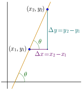 Slope Represented Graphically: The slope [latex]m =\frac{y_{2} - y_{1}}{x_{2} - x_{1}}[/latex] is calculated from the two points [latex]\left( x_1,y_1 \right)[/latex] and [latex]\left( x_2,y_2 \right)[/latex].
Now we’ll look at some graphs on a coordinate grid to find their slopes. In many cases, we can find slope by simply counting out the rise and the run. We start by locating two points on the line. If possible, we try to choose points with coordinates that are integers to make our calculations easier.
Example
Find the slope of the line shown on the coordinate plane below. Find the slope of the line: Notice the line is increasing so make sure to look for a slope that is positive.
Locate two points on the graph, choosing points whose coordinates are integers. We will use [latex](0, -3)[/latex] and [latex](5, 1)[/latex]. Starting with the point on the left, [latex](0, -3)[/latex], sketch a right triangle, going from the first point to the second point, [latex](5, 1)[/latex].
 Identify points on the line: Draw a triangle to help identify the rise and run.
Count the rise on the vertical leg of the triangle: [latex]4[/latex] units.
Count the run on the horizontal leg of the triangle: [latex]5[/latex] units. Use the slope formula to take the ratio of rise over run: [latex]\displaystyle \begin{align} m &= \frac{rise}{run} \\ &= \frac{4}{5} \end{align}[/latex] The slope of the line is [latex]\frac{4}{5}[/latex]. Notice that the slope is positive since the line slants upward from left to right.Example
Find the slope of the line shown on the coordinate plane below. Find the slope of the line: We can see the slope is decreasing, so be sure to look for a negative slope.
Locate two points on the graph. Look for points with coordinates that are integers. We can choose any points, but we will use [latex](0, 5)[/latex] and [latex](3, 3)[/latex].
 Identify two points on the line: The points [latex](0, 5)[/latex] and [latex](3, 3)[/latex] are on the line.
Direct and Inverse Variation
Two variables in direct variation have a linear relationship, while variables in inverse variation do not.Learning Objectives
Recognize examples of functions that vary directly and inverselyKey Takeaways
Key Points
- Two variables that change proportionally to one another are said to be in direct variation.
- The relationship between two directly proportionate variable can be represented by a linear equation in slope -intercept form, and is easily modeled using a linear graph.
- Inverse variation is the opposite of direct variation; two variables are said to be inversely proportional when a change is performed on one variable and the opposite happens to the other.
- The relationship between two inversely proportionate variables cannot be represented by a linear equation, and its graphical representation is not a line, but a hyperbola.
Key Terms
- hyperbola: A conic section formed by the intersection of a cone with a plane that intersects the base of the cone and is not tangent to the cone.
- proportional: At a constant ratio. Two magnitudes (numbers) are said to be proportional if the second varies in a direct relation arithmetically to the first.
Direct Variation
Simply put, two variables are in direct variation when the same thing that happens to one variable happens to the other. If [latex]x[/latex] and [latex]y[/latex] are in direct variation, and [latex]x[/latex] is doubled, then [latex]y[/latex] would also be doubled. The two variables may be considered directly proportional. For example, a toothbrush costs [latex]2[/latex] dollars. Purchasing [latex]5[/latex] toothbrushes would cost [latex]10[/latex] dollars, and purchasing [latex]10[/latex] toothbrushes would [latex]20[/latex] cost dollars. Thus we can say that the cost varies directly as the value of toothbrushes. Direct variation is represented by a linear equation, and can be modeled by graphing a line. Since we know that the relationship between two values is constant, we can give their relationship with: [latex]\displaystyle \frac{y}{x} = k[/latex] Where [latex]k[/latex] is a constant. Rewriting this equation by multiplying both sides by [latex]x[/latex] yields: [latex]\displaystyle y = kx[/latex] Notice that this is a linear equation in slope-intercept form, where the [latex]y[/latex]-intercept [latex]b[/latex] is equal to [latex]0[/latex]. Thus, any line passing through the origin represents a direct variation between [latex]x[/latex] and [latex]y[/latex]: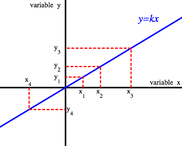 Directly Proportional Variables: The graph of [latex]y = kx[/latex] demonstrates an example of direct variation between two variables.
Revisiting the example with toothbrushes and dollars, we can define the [latex]x[/latex]-axis as number of toothbrushes and the [latex]y[/latex]-axis as number of dollars. Doing so, the variables would abide by the relationship:
[latex]\displaystyle \frac{y}{x} = 2[/latex] Any augmentation of one variable would lead to an equal augmentation of the other. For example, doubling [latex]y[/latex] would result in the doubling of [latex]x[/latex].Inverse Variation
Inverse variation is the opposite of direct variation. In the case of inverse variation, the increase of one variable leads to the decrease of another. In fact, two variables are said to be inversely proportional when an operation of change is performed on one variable and the opposite happens to the other. For example, if [latex]x[/latex] and [latex]y[/latex] are inversely proportional, if [latex]x[/latex] is doubled, then [latex]y[/latex] is halved. As an example, the time taken for a journey is inversely proportional to the speed of travel. If your car travels at a greater speed, the journey to your destination will be shorter. Knowing that the relationship between the two variables is constant, we can show that their relationship is: [latex]\displaystyle yx = k[/latex] Where [latex]k[/latex] is a constant known as the constant of proportionality. Note that as long as [latex]k[/latex] is not equal to [latex]0[/latex], neither [latex]x[/latex] nor [latex]y[/latex] can ever equal [latex]0[/latex] either. We can rearrange the above equation to place the variables on opposite sides: [latex]\displaystyle y=\frac{k}{x}[/latex] Notice that this is not a linear equation. It is impossible to put it in slope-intercept form. Thus, an inverse relationship cannot be represented by a line with constant slope. Inverse variation can be illustrated with a graph in the shape of a hyperbola, pictured below. Inversely Proportional Function: An inversely proportional relationship between two variables is represented graphically by a hyperbola.
Zeroes of Linear Functions
A zero, or [latex]x[/latex]-intercept, is the point at which a linear function's value will equal zero.Learning Objectives
Practice finding the zeros of linear functionsKey Takeaways
Key Points
- A zero is a point at which a function 's value will be equal to zero. Its coordinates are [latex](x,0)[/latex], where [latex]x[/latex] is equal to the zero of the graph.
- Zeros can be observed graphically or solved for algebraically.
- A linear function can have none, one, or infinitely many zeros. If the function is a horizontal line ( slope = [latex]0[/latex]), it will have no zeros unless its equation is [latex]y=0[/latex], in which case it will have infinitely many. If the line is non-horizontal, it will have one zero.
Key Terms
- zero: Also known as a root; an [latex]x[/latex] value at which the function of [latex]x[/latex] is equal to [latex]0[/latex].
- linear function: An algebraic equation in which each term is either a constant or the product of a constant and (the first power of) a single variable.
- y-intercept: A point at which a line crosses the [latex]y[/latex]-axis of a Cartesian grid.
Finding the Zeros of Linear Functions Graphically
Zeros can be observed graphically. An [latex]x[/latex]-intercept, or zero, is a property of many functions. Because the [latex]x[/latex]-intercept (zero) is a point at which the function crosses the [latex]x[/latex]-axis, it will have the value [latex](x,0)[/latex], where [latex]x[/latex] is the zero. All lines, with a value for the slope, will have one zero. To find the zero of a linear function, simply find the point where the line crosses the [latex]x[/latex]-axis.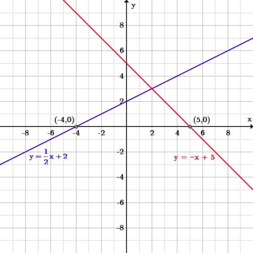 Zeros of linear functions: The blue line, [latex]y=\frac{1}{2}x+2[/latex], has a zero at [latex](-4,0)[/latex]; the red line, [latex]y=-x+5[/latex], has a zero at [latex](5,0)[/latex]. Since each line has a value for the slope, each line has exactly one zero.
Finding the Zeros of Linear Functions Algebraically
To find the zero of a linear function algebraically, set [latex]y=0[/latex] and solve for [latex]x[/latex]. The zero from solving the linear function above graphically must match solving the same function algebraically.Example: Find the zero of [latex]y=\frac{1}{2}x+2[/latex] algebraically
First, substitute [latex]0[/latex] for [latex]y[/latex]: [latex]\displaystyle 0=\frac{1}{2}x+2[/latex] Next, solve for [latex]x[/latex]. Subtract [latex]2[/latex] and then multiply by [latex]2[/latex], to obtain: [latex]\displaystyle \begin{align} \frac{1}{2}x&=-2\\ x&=-4 \end{align}[/latex] The zero is [latex](-4,0)[/latex]. This is the same zero that was found using the graphing method.Slope-Intercept Equations
The slope-intercept form of a line summarizes the information necessary to quickly construct its graph.Learning Objectives
Convert linear equations to slope-intercept form and explain why it is usefulKey Takeaways
Key Points
- The slope -intercept form of a line is given by [latex]y = mx + b[/latex] where [latex]m[/latex] is the slope of the line and [latex]b[/latex] is the [latex]y[/latex]-intercept.
- The constant [latex]b[/latex] is known as the [latex]y[/latex]-intercept. From slope- intercept form, when [latex]x=0[/latex], [latex]y=b[/latex], and the point [latex](0,b)[/latex] is the unique point on the line also on the [latex]y[/latex]-axis.
- To graph a line in slope-intercept form, first plot the [latex]y[/latex]-intercept, then use the value of the slope to locate a second point on the line. If the value of the slope is an integer, use a [latex]1[/latex] for the denominator.
- Use algebra to solve for [latex]y[/latex] if the equation is not written in slope-intercept form. Only then can the value of the slope and [latex]y[/latex]-intercept be located from the equation accurately.
Key Terms
- slope: The ratio of the vertical and horizontal distances between two points on a line; zero if the line is horizontal, undefined if it is vertical.
- y-intercept: A point at which a line crosses the [latex]y[/latex]-axis of a Cartesian grid.
Slope-Intercept Form
One of the most common representations for a line is with the slope-intercept form. Such an equation is given by [latex]y=mx+b[/latex], where [latex]x[/latex] and [latex]y[/latex] are variables and [latex]m[/latex] and [latex]b[/latex] are constants. When written in this form, the constant [latex]m[/latex] is the value of the slope and [latex]b[/latex] is the [latex]y[/latex]-intercept. Note that if [latex]m[/latex] is [latex]0[/latex], then [latex]y=b[/latex] represents a horizontal line. Note that this equation does not allow for vertical lines, since that would require that [latex]m[/latex] be infinite (undefined). However, a vertical line is defined by the equation [latex]x=c[/latex] for some constant [latex]c[/latex].Converting an Equation to Slope-Intercept Form
Writing an equation in slope-intercept form is valuable since from the form it is easy to identify the slope and [latex]y[/latex]-intercept. This assists in finding solutions to various problems, such as graphing, comparing two lines to determine if they are parallel or perpendicular and solving a system of equations.Example
Let's write an equation in slope-intercept form with [latex]m=-\frac{2}{3}[/latex], and [latex]b=3[/latex]. Simply substitute the values into the slope-intercept form to obtain: [latex]\displaystyle y=-\frac{2}{3}x+3[/latex] If an equation is not in slope-intercept form, solve for [latex]y[/latex] and rewrite the equation.Example
Let's write the equation [latex]3x+2y=-4[/latex] in slope-intercept form and identify the slope and [latex]y[/latex]-intercept. To solve the equation for [latex]y[/latex], first subtract [latex]3x[/latex] from both sides of the equation to get: [latex]\displaystyle 2y=-3x-4[/latex] Then divide both sides of the equation by [latex]2[/latex] to obtain: [latex]\displaystyle y=\frac{1}{2}(-3x-4)[/latex] Which simplifies to [latex]y=-\frac{3}{2}x-2[/latex]. Now that the equation is in slope-intercept form, we see that the slope [latex]m=-\frac{3}{2}[/latex], and the [latex]y[/latex]-intercept [latex]b=-2[/latex].Graphing an Equation in Slope-Intercept Form
We begin by constructing the graph of the equation in the previous example.Example
We construct the graph the line [latex]y=-\frac{3}{2}x-2[/latex] using the slope-intercept method. We begin by plotting the [latex]y[/latex]-intercept [latex]b=-2[/latex], whose coordinates are [latex](0,-2)[/latex]. The value of the slope dictates where to place the next point. Since the value of the slope is [latex]\frac{-3}{2}[/latex], the rise is [latex]-3[/latex] and the run is [latex]2[/latex]. This means that from the [latex]y[/latex]-intercept, [latex](0,-2)[/latex], move [latex]3[/latex] units down, and move [latex]2[/latex] units right. Thus we arrive at the point [latex](2,-5)[/latex] on the line. If the negative sign is placed with the denominator instead the slope would be written as [latex]\frac{3}{-2}[/latex], we can instead move up [latex]3[/latex] units and left [latex]2[/latex] units from the [latex]y[/latex]-intercept to arrive at the point [latex](-2,1)[/latex], also on the line.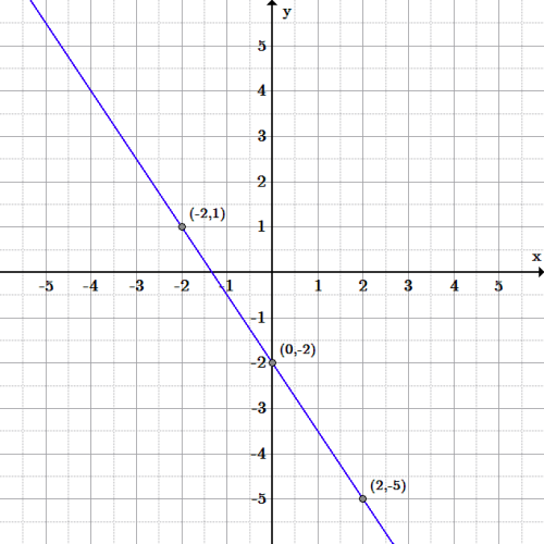 Slope-intercept graph: Graph of the line [latex]y=-\frac{3}{2}x-2[/latex].
Example
Let's graph the equation [latex]12x-6y-6=0[/latex]. First we solve the equation for [latex]y[/latex] by subtracting [latex]12x[/latex] to obtain: [latex]\displaystyle -6y-6=-12x[/latex] Next, add [latex]6[/latex] to get: [latex]\displaystyle -6y=-12x+6[/latex] Finally, divide all terms by [latex]-6[/latex] to get the slope-intercept form: [latex]\displaystyle y=2x-1[/latex] The slope is [latex]2[/latex], and the [latex]y[/latex]-intercept is [latex]-1[/latex]. Using this information, graphing is easy. Start by plotting the [latex]y[/latex]-intercept [latex](0,-1)[/latex], then use the value of the slope, [latex]\frac{2}{1}[/latex], to move up [latex]2[/latex] units and right [latex]1[/latex] unit.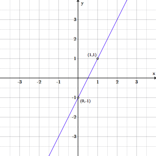 Slope-intercept graph: Graph of the line [latex]y=2x-1[/latex].
Point-Slope Equations
The point-slope equation is another way to represent a line; only the slope and a single point are needed.Learning Objectives
Use point-slope form to find the equation of a line passing through two points and verify that it is equivalent to the slope-intercept form of the equationKey Takeaways
Key Points
- The point - slope equation is given by [latex]y-y_{1}=m(x-x_{1})[/latex], where [latex](x_{1}, y_{1})[/latex] is any point on the line, and [latex]m[/latex] is the slope of the line.
- The point-slope equation requires that there is at least one point and the slope. If there are two points and no slope, the slope can be calculated from the two points first and then choose one of the two points to write the equation.
- The point-slope equation and slope-intercept equations are equivalent. It can be shown that given a point [latex](x_{1}, y_{1})[/latex] and slope [latex]m[/latex], the [latex]y[/latex]-intercept ([latex]b[/latex]) in the slope-intercept equation is [latex]y_{1}-mx_{1}[/latex].
Key Terms
- point-slope equation: An equation of a line given a point [latex](x_{1}, y_{1})[/latex] and a slope [latex]m[/latex]: [latex] y-y_{1}=m(x-x_{1})[/latex].
Point-Slope Equation
The point-slope equation is a way of describing the equation of a line. The point-slope form is ideal if you are given the slope and only one point, or if you are given two points and do not know what the [latex]y[/latex]-intercept is. Given a slope, [latex]m[/latex], and a point [latex](x_{1}, y_{1})[/latex], the point-slope equation is: [latex]\displaystyle y-y_{1}=m(x-x_{1})[/latex]Verify Point-Slope Form is Equivalent to Slope-Intercept Form
To show that these two equations are equivalent, choose a generic point [latex](x_{1}, y_{1})[/latex]. Plug in the generic point into the equation [latex]y=mx+b[/latex]. The equation is now, [latex]y_{1}=mx_{1}+b[/latex], giving us the ordered pair,[latex](x_{1}, mx_{1}+b)[/latex]. Then plug this point into the point-slope equation and solve for [latex]y[/latex] to get: [latex]\displaystyle y-(mx_{1}+b)=m(x-x_{1})[/latex] Distribute the negative sign through and distribute [latex]m[/latex] through [latex](x-x_{1})[/latex]: [latex]\displaystyle y-mx_{1}-b=mx-mx_{1}[/latex] Add [latex]mx_{1}[/latex] to both sides: [latex]\displaystyle y-mx_{1}+mx_{1}-b=mx-mx_{1}+mx_{1}[/latex] Combine like terms: [latex]\displaystyle y-b=mx[/latex] Add [latex]b[/latex] to both sides: [latex]\displaystyle y-b+b=mx+b[/latex] Combine like terms: [latex]\displaystyle y=mx+b[/latex] Therefore, the two equations are equivalent and either one can express an equation of a line depending on what information is given in the problem or what type of equation is requested in the problem.Example: Write the equation of a line in point-slope form, given a point [latex](2,1)[/latex] and slope [latex]-4[/latex], and convert to slope-intercept form
Write the equation of the line in point-slope form: [latex]\displaystyle y-1=-4(x-2)[/latex] To switch this equation into slope-intercept form, solve the equation for [latex]y[/latex]: [latex]\displaystyle y-1=-4(x-2)[/latex] Distribute [latex]-4[/latex]: [latex]\displaystyle y-1=-4x+8[/latex] Add [latex]1[/latex] to both sides: [latex]\displaystyle y=-4x+9[/latex] The equation has the same meaning whichever form it is in, and produces the same graph.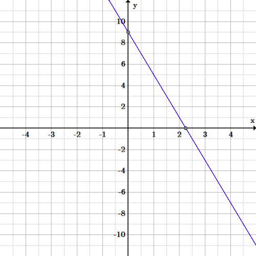 Line graph: Graph of the line [latex]y-1=-4(x-2)[/latex], through the point [latex](2,1)[/latex] with slope of [latex]-4[/latex], as well as the slope-intercept form, [latex]y=-4x+9[/latex].
Example: Write the equation of a line in point-slope form, given point [latex](-3,6)[/latex] and point [latex](1,2)[/latex], and convert to slope-intercept form
Since we have two points, but no slope, we must first find the slope: [latex]\displaystyle m=\frac{y_{2}-y_{1}}{x_{2}-x_{1}}[/latex] Substituting the values of the points: [latex]\displaystyle \begin{align} m&=\frac{-2-6}{1-(-3)}\\&=\frac{-8}{4}\\&=-2 \end{align}[/latex] Now choose either of the two points, such as [latex](-3,6)[/latex]. Plug this point and the calculated slope into the point-slope equation to get: [latex]\displaystyle y-6=-2[x-(-3)][/latex] Be careful if one of the coordinates is a negative. Distributing the negative sign through the parentheses, the final equation is: [latex]\displaystyle y-6=-2(x+3)[/latex] If you chose the other point, the equation would be: [latex]y+2=-2(x-1)[/latex] and either answer is correct. Next distribute [latex]-2[/latex]: [latex]\displaystyle y-6=-2x-6[/latex] Add [latex]6[/latex] to both sides: [latex]\displaystyle y=-2x[/latex] Again, the two forms of the equations are equivalent to each other and produce the same line. The only difference is the form that they are written in.Linear Equations in Standard Form
A linear equation written in standard form makes it easy to calculate the zero, or [latex]x[/latex]-intercept, of the equation.Learning Objectives
Explain the process and usefulness of converting linear equations to standard formKey Takeaways
Key Points
- The standard form of a linear equation is written as: [latex]Ax + By = C [/latex].
- The standard form is useful in calculating the zero of an equation. For a linear equation in standard form, if [latex]A[/latex] is nonzero, then the [latex]x[/latex]-intercept occurs at [latex]x = \frac{C}{A}[/latex].
Key Terms
- zero: Also known as a root, a zero is an [latex]x[/latex]-value at which the function of [latex]x[/latex] is equal to 0.
- slope-intercept form: A linear equation written in the form [latex]y = mx + b[/latex].
- y-intercept: A point at which a line crosses the y-axis of a Cartesian grid.
Standard Form
Standard form is another way of arranging a linear equation. In the standard form, a linear equation is written as: [latex]\displaystyle Ax + By = C [/latex] where [latex]A[/latex] and [latex]B[/latex] are both not equal to zero. The equation is usually written so that [latex]A \geq 0[/latex], by convention. The graph of the equation is a straight line, and every straight line can be represented by an equation in the standard form. For example, consider an equation in slope -intercept form: [latex]y = -12x +5[/latex]. In order to write this in standard form, note that we must move the term containing [latex]x[/latex] to the left side of the equation. We add [latex]12x[/latex] to both sides: [latex]\displaystyle y + 12x = 5[/latex] The equation is now in standard form.Using Standard Form to Find Zeroes
Recall that a zero is a point at which a function 's value will be equal to zero ([latex]y=0[/latex]), and is the [latex]x[/latex]-intercept of the function. We know that the y-intercept of a linear equation can easily be found by putting the equation in slope-intercept form. However, the zero of the equation is not immediately obvious when the linear equation is in this form. However, the zero, or [latex]x[/latex]-intercept of a linear equation can easily be found by putting it into standard form. For a linear equation in standard form, if [latex]A[/latex] is nonzero, then the [latex]x[/latex]-intercept occurs at [latex]x = \frac{C}{A}[/latex]. For example, consider the equation [latex]y + 12x = 5[/latex]. In this equation, the value of [latex]A[/latex] is 1, and the value of [latex]C[/latex] is 5. Therefore, the zero of the equation occurs at [latex]x = \frac{5}{1} = 5[/latex]. The zero is the point [latex](5, 0)[/latex]. Note that the [latex]y[/latex]-intercept and slope can also be calculated using the coefficients and constant of the standard form equation. If [latex]B[/latex] is non-zero, then the y-intercept, that is the y-coordinate of the point where the graph crosses the y-axis (where [latex]x[/latex] is zero), is [latex]\frac{C}{B}[/latex], and the slope of the line is [latex]-\frac{A}{B}[/latex].Example: Find the zero of the equation [latex]3(y - 2) = \frac{1}{4}x +3[/latex]
We must write the equation in standard form, [latex]Ax + By = C[/latex], which means getting the [latex]x[/latex] and [latex]y[/latex] terms on the left side, and the constants on the right side of the equation. Distribute the 3 on the left side: [latex]\displaystyle 3y - 6 = \frac{1}{4}x +3[/latex] Add 6 to both sides: [latex]\displaystyle 3y = \frac{1}{4}x + 9[/latex] Subtract [latex]\frac{1}{4}x[/latex] from both sides: [latex]\displaystyle 3y - \frac{1}{4}x = 9[/latex] Rearrange to [latex]Ax + By = C[/latex]: [latex]\displaystyle - \frac{1}{4}x+3y = 9[/latex] The equation is in standard form, and we can substitute the values for [latex]A[/latex] and [latex]C[/latex] into the formula for the zero: [latex]\displaystyle \begin{align} x &= \frac{C}{A} \\&= \frac{9}{-\frac{1}{4}} \\&= -36 \end{align}[/latex] The zero is [latex](-36, 0)[/latex].Licenses & Attributions
CC licensed content, Shared previously
- Curation and Revision. Authored by: Boundless.com. License: Public Domain: No Known Copyright.
CC licensed content, Specific attribution
- Algebra/Intercepts. Provided by: Wikibooks License: CC BY-SA: Attribution-ShareAlike.
- relation. Provided by: Wikipedia License: CC BY-SA: Attribution-ShareAlike.
- function. Provided by: Wikipedia License: CC BY-SA: Attribution-ShareAlike.
- Linear equation. Provided by: Wikipedia License: CC BY-SA: Attribution-ShareAlike.
- Algebra/Linear Equations and Functions. Provided by: Wikibooks License: CC BY-SA: Attribution-ShareAlike.
- Algebra/Slope. Provided by: Wikibooks License: CC BY-SA: Attribution-ShareAlike.
- variable. Provided by: Wiktionary License: CC BY-SA: Attribution-ShareAlike.
- Original figure by Julien Coyne. Licensed CC BY-SA 4.0. Provided by: Julien Coyne License: CC BY-SA: Attribution-ShareAlike.
- Basic Math. Provided by: OpenStax Located at: https://openstax.org/books/prealgebra/pages/1-introduction. License: CC BY: Attribution.
- Slope. Provided by: Wikipedia License: CC BY-SA: Attribution-ShareAlike.
- Original figure by Julien Coyne. Licensed CC BY-SA 4.0. Provided by: Julien Coyne License: CC BY-SA: Attribution-ShareAlike.
- Basic Math. Provided by: OpenStax Located at: https://openstax.org/books/prealgebra/pages/1-introduction. License: CC BY: Attribution.
- Basic Math. Provided by: OpenStax License: CC BY: Attribution.
- Basic Math. Provided by: OpenStax Located at: https://openstax.org/books/prealgebra/pages/1-introduction. License: CC BY: Attribution.
- Basic Math. Provided by: OpenStax License: CC BY: Attribution.
- Slope. Provided by: Wikipedia Located at: https://en.wikipedia.org/wiki/Slope#/media/File:Wiki_slope_in_2d.svg. License: CC BY-SA: Attribution-ShareAlike.
- Basic Math. Provided by: OpenStax Located at: https://openstax.org/books/prealgebra/pages/1-introduction. License: CC BY: Attribution.
- Slopes of Lines. Provided by: OpenStax License: CC BY: Attribution.
- Inverse Variation. Provided by: Boundless License: CC BY-SA: Attribution-ShareAlike.
- Direct Variation. Provided by: Boundless License: CC BY-SA: Attribution-ShareAlike.
- Combined Variation. Provided by: Boundless License: CC BY-SA: Attribution-ShareAlike.
- Proportionality (mathematics). Provided by: Wikipedia Located at: https://en.wikipedia.org/wiki/Proportionality_(mathematics). License: CC BY-SA: Attribution-ShareAlike.
- Original figure by Julien Coyne. Licensed CC BY-SA 4.0. Provided by: Julien Coyne License: CC BY-SA: Attribution-ShareAlike.
- Basic Math. Provided by: OpenStax Located at: https://openstax.org/books/prealgebra/pages/1-introduction. License: CC BY: Attribution.
- Basic Math. Provided by: OpenStax License: CC BY: Attribution.
- Basic Math. Provided by: OpenStax Located at: https://openstax.org/books/prealgebra/pages/1-introduction. License: CC BY: Attribution.
- Basic Math. Provided by: OpenStax License: CC BY: Attribution.
- Slope. Provided by: Wikipedia License: CC BY-SA: Attribution-ShareAlike.
- Basic Math. Provided by: OpenStax Located at: https://openstax.org/books/prealgebra/pages/1-introduction. License: CC BY: Attribution.
- Slopes of Lines. Provided by: OpenStax License: CC BY: Attribution.
- Inverse_proportionality_function_plot.gif. Provided by: Wikipedia License: Public Domain: No Known Copyright.
- Proportional_variables.svg. Provided by: Wikipedia License: Public Domain: No Known Copyright.
- Linear equation. Provided by: Wikipedia Located at: https://en.wikipedia.org/wiki/Linear_equation. License: CC BY-SA: Attribution-ShareAlike.
- Boundless. Provided by: Boundless Learning License: CC BY-SA: Attribution-ShareAlike.
- y-intercept. Provided by: Wiktionary License: CC BY-SA: Attribution-ShareAlike.
- linear function. Provided by: Wiktionary License: CC BY-SA: Attribution-ShareAlike.
- Original figure by Julien Coyne. Licensed CC BY-SA 4.0. Provided by: Julien Coyne License: CC BY-SA: Attribution-ShareAlike.
- Basic Math. Provided by: OpenStax Located at: https://openstax.org/books/prealgebra/pages/1-introduction. License: CC BY: Attribution.
- Basic Math. Provided by: OpenStax License: CC BY: Attribution.
- Basic Math. Provided by: OpenStax Located at: https://openstax.org/books/prealgebra/pages/1-introduction. License: CC BY: Attribution.
- Basic Math. Provided by: OpenStax License: CC BY: Attribution.
- Slope. Provided by: Wikipedia License: CC BY-SA: Attribution-ShareAlike.
- Basic Math. Provided by: OpenStax Located at: https://openstax.org/books/prealgebra/pages/1-introduction. License: CC BY: Attribution.
- Slopes of Lines. Provided by: OpenStax License: CC BY: Attribution.
- Inverse_proportionality_function_plot.gif. Provided by: Wikipedia License: Public Domain: No Known Copyright.
- Proportional_variables.svg. Provided by: Wikipedia License: Public Domain: No Known Copyright.
- Original figure by Julien Coyne. Licensed CC BY-SA 4.0. Provided by: Julien Coyne License: CC BY-SA: Attribution-ShareAlike.
- Algebra/Intercepts. Provided by: Wikibooks License: CC BY-SA: Attribution-ShareAlike.
- Algebra/Function Graphing. Provided by: Wikibooks License: CC BY-SA: Attribution-ShareAlike.
- Linear equation. Provided by: Wikipedia License: CC BY-SA: Attribution-ShareAlike.
- Algebra/Slope. Provided by: Wikibooks License: CC BY-SA: Attribution-ShareAlike.
- Algebra/Linear Equations and Functions. Provided by: Wikibooks License: CC BY-SA: Attribution-ShareAlike.
- y-intercept. Provided by: Wiktionary License: CC BY-SA: Attribution-ShareAlike.
- slope. Provided by: Wiktionary License: CC BY-SA: Attribution-ShareAlike.
- Original figure by Julien Coyne. Licensed CC BY-SA 4.0. Provided by: Julien Coyne License: CC BY-SA: Attribution-ShareAlike.
- Basic Math. Provided by: OpenStax Located at: https://openstax.org/books/prealgebra/pages/1-introduction. License: CC BY: Attribution.
- Basic Math. Provided by: OpenStax License: CC BY: Attribution.
- Basic Math. Provided by: OpenStax Located at: https://openstax.org/books/prealgebra/pages/1-introduction. License: CC BY: Attribution.
- Basic Math. Provided by: OpenStax License: CC BY: Attribution.
- Slope. Provided by: Wikipedia Located at: https://en.wikipedia.org/wiki/Slope#/media/File:Wiki_slope_in_2d.svg. License: CC BY-SA: Attribution-ShareAlike.
- Basic Math. Provided by: OpenStax Located at: https://openstax.org/books/prealgebra/pages/1-introduction. License: CC BY: Attribution.
- Slopes of Lines. Provided by: OpenStax License: CC BY: Attribution.
- Inverse_proportionality_function_plot.gif. Provided by: Wikipedia License: Public Domain: No Known Copyright.
- Proportional_variables.svg. Provided by: Wikipedia License: Public Domain: No Known Copyright.
- Original figure by Julien Coyne. Licensed CC BY-SA 4.0. Provided by: Julien Coyne License: CC BY-SA: Attribution-ShareAlike.
- Original figure by Julien Coyne. Licensed CC BY-SA 4.0. Provided by: Julien Coyne License: CC BY-SA: Attribution-ShareAlike.
- Original figure by Julien Coyne. Licensed CC BY-SA 4.0. Provided by: Julien Coyne License: CC BY-SA: Attribution-ShareAlike.
- Linear equation. Provided by: Wikipedia License: CC BY-SA: Attribution-ShareAlike.
- Algebra/Function Graphing. Provided by: Wikibooks License: CC BY-SA: Attribution-ShareAlike.
- Boundless. Provided by: Boundless Learning License: CC BY-SA: Attribution-ShareAlike.
- Original figure by Julien Coyne. Licensed CC BY-SA 4.0. Provided by: Julien Coyne License: CC BY-SA: Attribution-ShareAlike.
- Basic Math. Provided by: OpenStax Located at: https://openstax.org/books/prealgebra/pages/1-introduction. License: CC BY: Attribution.
- Basic Math. Provided by: OpenStax License: CC BY: Attribution.
- Basic Math. Provided by: OpenStax Located at: https://openstax.org/books/prealgebra/pages/1-introduction. License: CC BY: Attribution.
- Basic Math. Provided by: OpenStax License: CC BY: Attribution.
- Slope. Provided by: Wikipedia Located at: https://en.wikipedia.org/wiki/Slope#/media/File:Wiki_slope_in_2d.svg. License: CC BY-SA: Attribution-ShareAlike.
- Basic Math. Provided by: OpenStax Located at: https://openstax.org/books/prealgebra/pages/1-introduction. License: CC BY: Attribution.
- Slopes of Lines. Provided by: OpenStax License: CC BY: Attribution.
- Inverse_proportionality_function_plot.gif. Provided by: Wikipedia License: Public Domain: No Known Copyright.
- Proportional_variables.svg. Provided by: Wikipedia License: Public Domain: No Known Copyright.
- Original figure by Julien Coyne. Licensed CC BY-SA 4.0. Provided by: Julien Coyne License: CC BY-SA: Attribution-ShareAlike.
- Original figure by Julien Coyne. Licensed CC BY-SA 4.0. Provided by: Julien Coyne License: CC BY-SA: Attribution-ShareAlike.
- Original figure by Julien Coyne. Licensed CC BY-SA 4.0. Provided by: Julien Coyne License: CC BY-SA: Attribution-ShareAlike.
- Original figure by Julien Coyne. Licensed CC BY-SA 4.0. Provided by: Julien Coyne License: CC BY-SA: Attribution-ShareAlike.
- Linear equation. Provided by: Wikipedia License: CC BY-SA: Attribution-ShareAlike.
- Zeroes of Linear Equations. Provided by: Boundless License: CC BY-SA: Attribution-ShareAlike.
- Original figure by Julien Coyne. Licensed CC BY-SA 4.0. Provided by: Julien Coyne License: CC BY-SA: Attribution-ShareAlike.
- Basic Math. Provided by: OpenStax Located at: https://openstax.org/books/prealgebra/pages/1-introduction. License: CC BY: Attribution.
- Basic Math. Provided by: OpenStax License: CC BY: Attribution.
- Basic Math. Provided by: OpenStax Located at: https://openstax.org/books/prealgebra/pages/1-introduction. License: CC BY: Attribution.
- Basic Math. Provided by: OpenStax License: CC BY: Attribution.
- Slope. Provided by: Wikipedia Located at: https://en.wikipedia.org/wiki/Slope#/media/File:Wiki_slope_in_2d.svg. License: CC BY-SA: Attribution-ShareAlike.
- Basic Math. Provided by: OpenStax Located at: https://openstax.org/books/prealgebra/pages/1-introduction. License: CC BY: Attribution.
- Slopes of Lines. Provided by: OpenStax License: CC BY: Attribution.
- Inverse_proportionality_function_plot.gif. Provided by: Wikipedia License: Public Domain: No Known Copyright.
- Proportional_variables.svg. Provided by: Wikipedia License: Public Domain: No Known Copyright.
- Original figure by Julien Coyne. Licensed CC BY-SA 4.0. Provided by: Julien Coyne License: CC BY-SA: Attribution-ShareAlike.
- Original figure by Julien Coyne. Licensed CC BY-SA 4.0. Provided by: Julien Coyne License: CC BY-SA: Attribution-ShareAlike.
- Original figure by Julien Coyne. Licensed CC BY-SA 4.0. Provided by: Julien Coyne License: CC BY-SA: Attribution-ShareAlike.
- Original figure by Julien Coyne. Licensed CC BY-SA 4.0. Provided by: Julien Coyne License: CC BY-SA: Attribution-ShareAlike.
