
Linear and Geometric Growth
Constant change is the defining characteristic of linear growth. Plotting coordinate pairs associated with constant change will result in a straight line, the shape of linear growth. In this section, we will formalize a way to describe linear growth using mathematical terms and concepts. By the end of this section, you will be able to write both a recursive and explicit equations for linear growth given starting conditions, or a constant of change. You will also be able to recognize the difference between linear and geometric growth given a graph or an equation.
Learning Objectives
- Determine whether data or a scenario describe linear or geometric growth
- Identify growth rates, initial values, or point values expressed verbally, graphically, or numerically, and translate them into a format usable in calculation
- Calculate recursive and explicit equations for linear and geometric growth given sufficient information, and use those equations to make predictions
Linear (Algebraic) Growth
Predicting Growth
Marco is a collector of antique soda bottles. His collection currently contains 437 bottles. Every year, he budgets enough money to buy 32 new bottles. Can we determine how many bottles he will have in 5 years, and how long it will take for his collection to reach 1000 bottles? While you could probably solve both of these questions without an equation or formal mathematics, we are going to formalize our approach to this problem to provide a means to answer more complicated questions.
Suppose that Pn represents the number, or population, of bottles Marco has after n years. So P0 would represent the number of bottles now, P1 would represent the number of bottles after 1 year, P2 would represent the number of bottles after 2 years, and so on. We could describe how Marco’s bottle collection is changing using:
While you could probably solve both of these questions without an equation or formal mathematics, we are going to formalize our approach to this problem to provide a means to answer more complicated questions.
Suppose that Pn represents the number, or population, of bottles Marco has after n years. So P0 would represent the number of bottles now, P1 would represent the number of bottles after 1 year, P2 would represent the number of bottles after 2 years, and so on. We could describe how Marco’s bottle collection is changing using:
P0 = 437
Pn = Pn-1 + 32
This is called a recursive relationship. A recursive relationship is a formula which relates the next value in a sequence to the previous values. Here, the number of bottles in year n can be found by adding 32 to the number of bottles in the previous year, Pn-1. Using this relationship, we could calculate:P1 = P0 + 32 = 437 + 32 = 469
P2 = P1 + 32 = 469 + 32 = 501
P3 = P2 + 32 = 501 + 32 = 533
P4 = P3 + 32 = 533 + 32 = 565
P5 = P4 + 32 = 565 + 32 = 597
We have answered the question of how many bottles Marco will have in 5 years.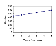 However, solving how long it will take for his collection to reach 1000 bottles would require a lot more calculations.
While recursive relationships are excellent for describing simply and cleanly how a quantity is changing, they are not convenient for making predictions or solving problems that stretch far into the future. For that, a closed or explicit form for the relationship is preferred. An explicit equation allows us to calculate Pn directly, without needing to know Pn-1. While you may already be able to guess the explicit equation, let us derive it from the recursive formula. We can do so by selectively not simplifying as we go:
However, solving how long it will take for his collection to reach 1000 bottles would require a lot more calculations.
While recursive relationships are excellent for describing simply and cleanly how a quantity is changing, they are not convenient for making predictions or solving problems that stretch far into the future. For that, a closed or explicit form for the relationship is preferred. An explicit equation allows us to calculate Pn directly, without needing to know Pn-1. While you may already be able to guess the explicit equation, let us derive it from the recursive formula. We can do so by selectively not simplifying as we go:
P1 = 437 + 32 = 437 + 1(32)
P2 = P1 + 32 = 437 + 32 + 32 = 437 + 2(32)
P3 = P2 + 32 = (437 + 2(32)) + 32 = 437 + 3(32)
P4 = P3 + 32 = (437 + 3(32)) + 32 = 437 + 4(32)
You can probably see the pattern now, and generalize thatPn = 437 + n(32) = 437 + 32n
Using this equation, we can calculate how many bottles he’ll have after 5 years:P5 = 437 + 32(5) = 437 + 160 = 597
We can now also solve for when the collection will reach 1000 bottles by substituting in 1000 for Pn and solving for n1000 = 437 + 32n
563 = 32n
n = 563/32 = 17.59
So Marco will reach 1000 bottles in 18 years. The steps of determining the formula and solving the problem of Marco's bottle collection are explained in detail in the following videos. https://youtu.be/SJcAjN-HL_I https://youtu.be/4Two_oduhrA https://youtu.be/pZ4u3j8Vmzo In this example, Marco’s collection grew by the same number of bottles every year. This constant change is the defining characteristic of linear growth. Plotting the values we calculated for Marco’s collection, we can see the values form a straight line, the shape of linear growth.Linear Growth
If a quantity starts at size P0 and grows by d every time period, then the quantity after n time periods can be determined using either of these relations:Recursive form
Pn = Pn-1 + d
Explicit form
Pn = P0 + d n
In this equation, d represents the common difference – the amount that the population changes each time n increases by 1.Connection to Prior Learning: Slope and Intercept
You may recognize the common difference, d, in our linear equation as slope. In fact, the entire explicit equation should look familiar – it is the same linear equation you learned in algebra, probably stated as y = mx + b. In the standard algebraic equation y = mx + b, b was the y-intercept, or the y value when x was zero. In the form of the equation we’re using, we are using P0 to represent that initial amount. In the y = mx + b equation, recall that m was the slope. You might remember this as “rise over run,” or the change in y divided by the change in x. Either way, it represents the same thing as the common difference, d, we are using – the amount the output Pn changes when the input n increases by 1. The equations y = mx + b and Pn = P0 + d n mean the same thing and can be used the same ways. We’re just writing it somewhat differently.Examples
The population of elk in a national forest was measured to be 12,000 in 2003, and was measured again to be 15,000 in 2007. If the population continues to grow linearly at this rate, what will the elk population be in 2014?Answer: To begin, we need to define how we’re going to measure n. Remember that P0 is the population when n = 0, so we probably don’t want to literally use the year 0. Since we already know the population in 2003, let us define n = 0 to be the year 2003. Then P0 = 12,000. Next we need to find d. Remember d is the growth per time period, in this case growth per year. Between the two measurements, the population grew by 15,000-12,000 = 3,000, but it took 2007-2003 = 4 years to grow that much. To find the growth per year, we can divide: 3000 elk / 4 years = 750 elk in 1 year. Alternatively, you can use the slope formula from algebra to determine the common difference, noting that the population is the output of the formula, and time is the input. [latex-display]d=slope=\frac{\text{changeinoutput}}{\text{changeininput}}=\frac{15,000-12,000}{2007-2003}=\frac{3000}{4}=750[/latex-display] We can now write our equation in whichever form is preferred.
Recursive form
P0 = 12,000
Pn = Pn-1 + 750
Explicit form
Pn = 12,000 + 750n
To answer the question, we need to first note that the year 2014 will be n = 11, since 2014 is 11 years after 2003. The explicit form will be easier to use for this calculation:P11 = 12,000 + 750(11) = 20,250 elk
View more about this example here. https://youtu.be/J1XqqlKzYGsGasoline consumption in the US has been increasing steadily. Consumption data from 1992 to 2004 is shown below.[footnote]http://www.bts.gov/publications/national_transportation_statistics/2005/html/table_04_10.html[/footnote] Find a model for this data, and use it to predict consumption in 2016. If the trend continues, when will consumption reach 200 billion gallons?
| Year | '92 | '93 | '94 | '95 | '96 | '97 | '98 | '99 | '00 | '01 | '02 | '03 | '04 |
| Consumption (billion of gallons) | 110 | 111 | 113 | 116 | 118 | 119 | 123 | 125 | 126 | 128 | 131 | 133 | 136 |
Answer:
Plotting this data, it appears to have an approximately linear relationship:
 While there are more advanced statistical techniques that can be used to find an equation to model the data, to get an idea of what is happening, we can find an equation by using two pieces of the data – perhaps the data from 1993 and 2003.
Letting n = 0 correspond with 1993 would give P0 = 111 billion gallons.
To find d, we need to know how much the gas consumption increased each year, on average. From 1993 to 2003 the gas consumption increased from 111 billion gallons to 133 billion gallons, a total change of 133 – 111 = 22 billion gallons, over 10 years. This gives us an average change of 22 billion gallons / 10 year = 2.2 billion gallons per year.
Equivalently,
[latex]d=slope=\frac{\text{changeinoutput}}{\text{changeininput}}=\frac{133-111}{10-0}=\frac{22}{10}=2.2[/latex]billion gallons per year
We can now write our equation in whichever form is preferred.
While there are more advanced statistical techniques that can be used to find an equation to model the data, to get an idea of what is happening, we can find an equation by using two pieces of the data – perhaps the data from 1993 and 2003.
Letting n = 0 correspond with 1993 would give P0 = 111 billion gallons.
To find d, we need to know how much the gas consumption increased each year, on average. From 1993 to 2003 the gas consumption increased from 111 billion gallons to 133 billion gallons, a total change of 133 – 111 = 22 billion gallons, over 10 years. This gives us an average change of 22 billion gallons / 10 year = 2.2 billion gallons per year.
Equivalently,
[latex]d=slope=\frac{\text{changeinoutput}}{\text{changeininput}}=\frac{133-111}{10-0}=\frac{22}{10}=2.2[/latex]billion gallons per year
We can now write our equation in whichever form is preferred.
Recursive form
P0 = 111
Pn = Pn-1 + 2.2
Explicit form
Pn = 111 + 2.2n
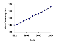 Calculating values using the explicit form and plotting them with the original data shows how well our model fits the data.
We can now use our model to make predictions about the future, assuming that the previous trend continues unchanged. To predict the gasoline consumption in 2016:
Calculating values using the explicit form and plotting them with the original data shows how well our model fits the data.
We can now use our model to make predictions about the future, assuming that the previous trend continues unchanged. To predict the gasoline consumption in 2016:
n = 23 (2016 – 1993 = 23 years later)
P23 = 111 + 2.2(23) = 161.6
Our model predicts that the US will consume 161.6 billion gallons of gasoline in 2016 if the current trend continues. To find when the consumption will reach 200 billion gallons, we would set Pn = 200, and solve for n:Pn = 200 Replace Pn with our model
111 + 2.2n = 200 Subtract 111 from both sides
2.2n = 89 Divide both sides by 2.2
n = 40.4545
This tells us that consumption will reach 200 billion about 40 years after 1993, which would be in the year 2033. The steps for reaching this answer are detailed in the following video. https://youtu.be/ApFxDWd6IbEThe cost, in dollars, of a gym membership for n months can be described by the explicit equation Pn = 70 + 30n. What does this equation tell us?
Answer: The value for P0 in this equation is 70, so the initial starting cost is $70. This tells us that there must be an initiation or start-up fee of $70 to join the gym. The value for d in the equation is 30, so the cost increases by $30 each month. This tells us that the monthly membership fee for the gym is $30 a month.
The explanation for this example is detailed below. https://youtu.be/0Uwz5dmLTtkTry It Now
The number of stay-at-home fathers in Canada has been growing steadily[footnote]http://www.fira.ca/article.php?id=140[/footnote]. While the trend is not perfectly linear, it is fairly linear. Use the data from 1976 and 2010 to find an explicit formula for the number of stay-at-home fathers, then use it to predict the number in 2020.| Year | 1976 | 1984 | 1991 | 2000 | 2010 |
| # of Stay -at-home fathers | 20610 | 28725 | 43530 | 47665 | 53555 |
Answer:
Examples
A friend is using the equation Pn = 4600(1.072)n to predict the annual tuition at a local college. She says the formula is based on years after 2010. What does this equation tell us?Answer: In the equation, P0 = 4600, which is the starting value of the tuition when n = 0. This tells us that the tuition in 2010 was $4,600. The growth multiplier is 1.072, so the growth rate is 0.072, or 7.2%. This tells us that the tuition is expected to grow by 7.2% each year. Putting this together, we could say that the tuition in 2010 was $4,600, and is expected to grow by 7.2% each year.
View the following to see this example worked out. https://youtu.be/T8Yz94De5UMIn 1990, residential energy use in the US was responsible for 962 million metric tons of carbon dioxide emissions. By the year 2000, that number had risen to 1182 million metric tons[footnote]http://www.eia.doe.gov/oiaf/1605/ggrpt/carbon.html[/footnote]. If the emissions grow exponentially and continue at the same rate, what will the emissions grow to by 2050?
Answer: Similar to before, we will correspond n = 0 with 1990, as that is the year for the first piece of data we have. That will make P0 = 962 (million metric tons of CO2). In this problem, we are not given the growth rate, but instead are given that P10 = 1182. When n = 10, the explicit equation looks like:
P10 = (1+r)10 P0
We know the value for P0, so we can put that into the equation:P10 = (1+r)10 962
We also know that P10 = 1182, so substituting that in, we get1182 = (1+r)10 962
We can now solve this equation for the growth rate, r. Start by dividing by 962.[latex]\frac{1182}{962}={{(1+r)}^{10}}[/latex] Take the 10th root of both sides
[latex]\sqrt[10]{\frac{1182}{962}}=1+r[/latex] Subtract 1 from both sides
[latex]r=\sqrt[10]{\frac{1182}{962}}-1=0.0208[/latex] = 2.08%
So if the emissions are growing exponentially, they are growing by about 2.08% per year. We can now predict the emissions in 2050 by finding P60P60 = (1+0.0208)60 962 = 3308.4 million metric tons of CO2 in 2050
View more about this example here. https://youtu.be/9Zu2uONfLkQRounding
As a note on rounding, notice that if we had rounded the growth rate to 2.1%, our calculation for the emissions in 2050 would have been 3347. Rounding to 2% would have changed our result to 3156. A very small difference in the growth rates gets magnified greatly in exponential growth. For this reason, it is recommended to round the growth rate as little as possible. If you need to round, keep at least three significant digits - numbers after any leading zeros. So 0.4162 could be reasonably rounded to 0.416. A growth rate of 0.001027 could be reasonably rounded to 0.00103.Evaluating roots on the calculator
In the previous example, we had to calculate the 10th root of a number. This is different than taking the basic square root, √. Many scientific calculators have a button for general roots. It is typically labeled like:[latex]\sqrt[y]{x}[/latex]
To evaluate the 3rd root of 8, for example, we’d either type 3 [latex]\sqrt[x]{{}}[/latex] 8, or 8 [latex]\sqrt[x]{{}}[/latex] 3, depending on the calculator. Try it on yours to see which to use – you should get an answer of 2. If your calculator does not have a general root button, all is not lost. You can instead use the property of exponents which states that:[latex]\sqrt[n]{a}={a}^{\frac{1}{2}}[/latex].
So, to compute the 3rd root of 8, you could use your calculator’s exponent key to evaluate 81/3. To do this, type:8 yx ( 1 ÷ 3 )
The parentheses tell the calculator to divide 1/3 before doing the exponent.Try It Now
The number of users on a social networking site was 45 thousand in February when they officially went public, and grew to 60 thousand by October. If the site is growing exponentially, and growth continues at the same rate, how many users should they expect two years after they went public?Answer: Here we will measure n in months rather than years, with n = 0 corresponding to the February when they went public. This gives [latex]P_0= 45[/latex] thousand. October is 8 months later, so [latex]P_8= 60[/latex]. [latex-display]P_8=(1+r)^{8}P_0[/latex-display] [latex-display]60=(1+r)^{8}45[/latex-display] [latex-display]\frac{60}{45}=(1+r)^8[/latex-display] [latex-display]\sqrt[8]{\frac{60}{45}}=1+r[/latex-display] [latex-display]r=\sqrt[8]{\frac{60}{45}}-1=0.0366\text{ or }3.66%[/latex-display] The general explicit equation is [latex]P_n =(1.0366)^{n}45[/latex]. Predicting 24 months after they went public gives [latex]P_{24}=(1.0366)^{24}45=106.63[/latex] thousand users.
Example
Looking back at the last example, for the sake of comparison, what would the carbon emissions be in 2050 if emissions grow linearly at the same rate?Answer: Again we will get n = 0 correspond with 1990, giving P0 = 962. To find d, we could take the same approach as earlier, noting that the emissions increased by 220 million metric tons in 10 years, giving a common difference of 22 million metric tons each year. Alternatively, we could use an approach similar to that which we used to find the exponential equation. When n = 10, the explicit linear equation looks like:
P10 = P0 + 10d
We know the value for P0, so we can put that into the equation:P10 = 962 + 10d
Since we know that P10 = 1182, substituting that in we get1182 = 962 + 10d
We can now solve this equation for the common difference, d.1182 – 962 = 10d
220 = 10d
d = 22
This tells us that if the emissions are changing linearly, they are growing by 22 million metric tons each year. Predicting the emissions in 2050,P60 = 962 + 22(60) = 2282 million metric tons.
You will notice that this number is substantially smaller than the prediction from the exponential growth model. Calculating and plotting more values helps illustrate the differences.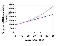 A demonstration of this example can be seen in the following video.
https://youtu.be/yiuZoiRMtYM
A demonstration of this example can be seen in the following video.
https://youtu.be/yiuZoiRMtYM
- Find more than two pieces of data. Plot the values, and look for a trend. Does the data appear to be changing like a line, or do the values appear to be curving upwards?
- Consider the factors contributing to the data. Are they things you would expect to change linearly or exponentially? For example, in the case of carbon emissions, we could expect that, absent other factors, they would be tied closely to population values, which tend to change exponentially.
Licenses & Attributions
CC licensed content, Original
- Introduction and Learning Outcomes. Provided by: Lumen Learning License: CC BY: Attribution.
- Revision and Adaptation. Provided by: Lumen Learning License: CC BY: Attribution.
CC licensed content, Shared previously
- Growth. Authored by: bykst. License: Public Domain: No Known Copyright.
- Math in Society. Authored by: David Lippman. Located at: http://www.opentextbookstore.com/mathinsociety/. License: CC BY-SA: Attribution-ShareAlike.
- Feira Tom Jobim - BH. Authored by: Antonio Thomas Koenigkam Oliveira. Located at: https://www.flickr.com/photos/antoniothomas/15186624687/. License: CC BY: Attribution.
- Linear Growth Part 1. Authored by: OCLPhase2's channel. License: CC BY: Attribution.
- Linear Growth Part 2. Authored by: OCLPhase2's channel. License: CC BY: Attribution.
- Linear Growth Part 3. Authored by: OCLPhase2's channel. License: CC BY: Attribution.
- Linear Growth - Elk. Authored by: OCLPhase2's channel. License: CC BY: Attribution.
- Finding linear model for gas consumption. Authored by: OCLPhase2's channel. License: CC BY: Attribution.
- Interpreting a linear model. Authored by: OCLPhase2's channel. License: CC BY: Attribution.
- Linear model breakdown. Authored by: OCLPhase2's channel. License: CC BY: Attribution.
- Question ID 6594. Authored by: Lippman, David. License: CC BY: Attribution. License terms: IMathAS Community License CC-BY + GPL.
- calf-fish-lake-pond-river. Authored by: Pexels. License: CC0: No Rights Reserved.
- Exponential Growth Model Part 1. Authored by: OCLPhase2's channel. License: CC BY: Attribution.
- Exponential Growth Model Part 2. Authored by: OCLPhase2's channel. License: CC BY: Attribution.
- Predicting future population using an exponential model. Authored by: OCLPhase2's channel. License: CC BY: Attribution.
- Interpreting an Exponential Equation. Authored by: OCLPhase2's channel. License: CC BY: Attribution.
- Finding an Exponential Model. Authored by: OCLPhase2's channel. License: CC BY: Attribution.
- Comparing exponential to linear growth. Authored by: OCLPhase2's channel. License: CC BY: Attribution.
- Question ID 6598. Authored by: Lippman, David. License: CC BY: Attribution. License terms: IMathAS Community License CC-BY + GPL.
